Content from Opening and Checking an Image
Last updated on 2025-03-21 | Edit this page
Overview
Questions
- How do I open an image file in Python for processing?
- How can I explore an image once it’s open?
Objectives
- Open an image with skimage
- Discuss how to open proprietary image formats
- Display an opened image to the screen
Opening an image
At its core, an image is a multidimensional array of numbers, and as
such can be opened by programs and libraries designed for working with
this kind of data. For Python, one such library is scikit-image. This
library provides a function called imread that we can use
to load an image into memory. In a new notebook cell:
If you saved your images to a different location, you will need to change the file path provided to imread accordingly. Paths will be relative to the location of your .ipynb notebook file.
To view things in Python, usually we use print().
However if we try to print this image to the Jupyter console, instead of
the image we get something that may be unexpected:
OUTPUT
> print(image)
array([[[ 16,  50,   0],
        [ 15,  44,   0],
        [ 18,  40,   1],
        ...,
        [  1,  15,   2],
        [  1,  15,   2],
        [  1,  15,   2]]], dtype=uint8)
Python has loaded and stored the image as a Numpy array
object of numbers, and print() displays the string
representation or textual form of the data passed to it, which is why we
get a matrix of numbers printed to the screen.
If we want to see what the image looks like, we need tell Python to
display it as an image. We can do this with the imshow
function from matplotlib, which you may already be familiar with as a
library for drawing plots and graphs, but it can also display
images.
PYTHON
import matplotlib.pyplot as plt

plt.set_cmap('gray')  # by default, single-channel images will now be displayed in greyscale
plt.imshow(image)
You should now see the image displayed below the current cell:
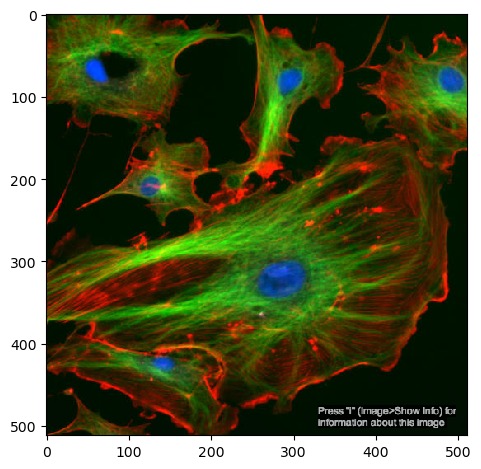
Since images are multi-dimensional arrays of numbers, we can apply statistical functions to them and extract some basic metrics. Numpy arrays have methods for several of these already, including the image’s shape, data type and minimum/maximum values:
PYTHON
print(image.shape, image.dtype, image.min(), image.max())
# returns: (512, 512, 3) uint8 0 255
This shows that the image has a data type of uint8, it contains
values between 0 and 255 and that it is in three dimensions. We can
reasonably infer that the two 512 numbers are the X and Y
axes. The third axis in most cases will represent a number of
channels.
We can select a single channel by indexing the array:
Here, we select the entire X and Y axes using : with no
numbers around them, and the last channel (remember that Python counts
from 0).
Channels, series and stacks
Images can consist of more than two axes. The first two axes are usually X and Y, but if there is a third axis, then this could be one of several things:
- Channel - the image shows different features in the same 2D space. One common example is cell images with different staining for nuclei and membranes, expressed as different colours.
- Time series - the image is a collection of 2D frames taken at different points in time.
- Z-stack - essentially a series of 2D images piled up on top of each other in 3D space.
It’s usually easy enough to tell that you’re looking at a colour channel from looking at the image directly, but it may be more difficult to to distinguish a Z or a timepoint axis from the data alone. If you don’t know exactly how the images were generated, it’s a good idea to consult documentation or metadata.
Exercise 1: Loading an image
Load the test image ‘FluorescentCells_3channel.tif’:
- Try the same as the example above, but display one of the other channels
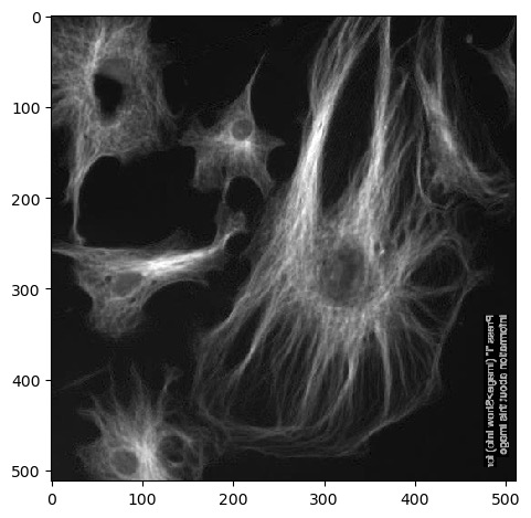
- Save your single channel to a variable. What happens if you run
imshowonchannel.T? - How can we select part of the image, i.e. crop it? Remember that to do this, we need to select a subset of the X and/or Y axes.
Other channels can be loaded with image[:, :, x], where
image is the variable the image is saved to and
x is the index of a channel to retrieve.
Next we can use .T to return a
transposed version of the image. Running
imshow() on this results in an image that is flipped
90°:
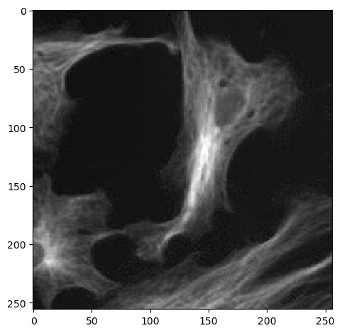
Remember that Numpy arrays can be sliced and indexed the same way as
lists, strings and tuples. Up to this point we’ve been using
: to select an entire axis, but we can give it start and
end bounds to select part of the X and Y axes, like:
Numpy arrays have many more methods available for checking them. Here are just a few to start with:
Object size
Note that some of these are functions and need to be called with
brackets(()), whereas others are simply attributes that do
not.
Exercise 2: Memory check
How much memory did it take to load FluorescentCells_3channel.tif?
Running image.nbytes shows that it takes up 786432
bytes, or ~786 kilobytes, or ~0.7 megabytes.
Displaying one channel at a time
We’ve seen from exercise 1 that we can view single channels by indexing the array. We can also show all channels together using a matplotlib figure:
PYTHON
import matplotlib.pyplot as plt
plt.figure(figsize=(12, 6))  # figure size, in inches
nchannels = 3

for i in range(nchannels):
    # Use subplot() to create a multi-image figure with 1 row and 3 columns. We need to increment i by 1
    # because range() counts from 0 but subplot() assumes you're counting from 1.
    plt.subplot(1, nchannels, i+1)
    plt.imshow(image[:, :, i])
    plt.title('Channel ' + str(i))  # add a plot title
    plt.axis(False)              # we just want to show the image, so turn off the axis labels

plt.show()
Histograms
Another useful metric in image analysis is an image’s histogram. This can be plotted by flattening the image and passing it to matplotlib:
First, we need to select a single channel - since different channels
may represent different cell organelles or points in time, we need to
ensure that we are comparing like with like. We also need
flatten() because we don’t care about the arrangement of
the pixels, we just want to sort their values values into bins. Finally,
we can use bins to control how many bins the data is split
into.
Exercise 3: Histograms
Combine the usage of matplotlib.pyplot.hist() and
matplotlib.pyplot.figure() introduced above above and plot
a histogram of each of the three channels in
FluorescentCells_3channel.tif.
Starting with displaying a single histogram for one channel:
PYTHON
channel_idx = 0
channel = image[:, :, channel_idx]
plt.hist(channel.flatten(), bins=255)
plt.title('Channel ' + str(channel_idx))
plt.show()
We could call this three times, each with a different value for
channel_idx, or we can use a for loop:
PYTHON
plt.figure(figsize=(12, 6))  # figure size, in inches
nchannels = image.shape[-1]

for i in range(nchannels):
    channel = image[:, :, i]

    plt.subplot(1, nchannels, i+1)
    plt.hist(channel.flatten(), bins=255)
    plt.title('Channel ' + str(i))  # add a plot title

plt.show()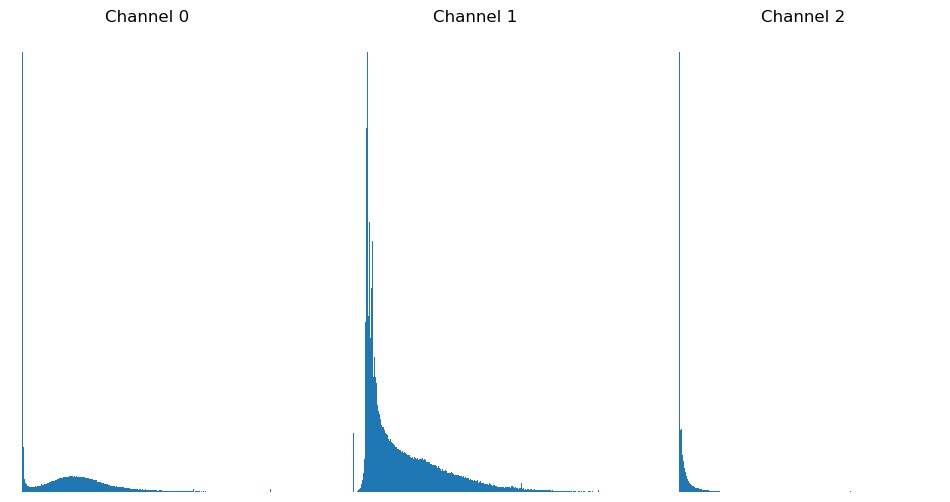
Proprietary formats
Images can come in many formats, but for many of the common ones such as TIFF, PNG and BMP, skimage is smart enough to know how to read each one.
Some image formats are associated with specific instruments or
equipment and require specialised packages to open. Depending on your
system, these may already be available via import the same
as any other Python package. If not, then these should be installed into
whatever Python instance you are using.
If using JupyterHub or JupyterLab, go to ‘New’ -> ‘Terminal’. This
will open a shell session in a new browser tab, where you can run
pip install commands.
Carl Zeiss .czi
Images in .czi format can be opened with the czifile
library. In the Terminal you opened above:
Leica .lif
Exercise 4: Proprietary formats
Load the nd2 package and use it to read the test file ‘Ersi_organoid_WT2.nd2’. Install it if you need to.
What axes are present in the image? Which look most likely to be the
X and Y axes? Use imshow to display a single frame from the
image.
If not already present, the nd2 package can be installed in the
Terminal with pip install nd2. According to its linked
documentation, it has an imread function that works in a
similar way to the one in skimage, and returns a numpy multidimensional
array that we can work with the same way we have before:
PYTHON
import nd2
image = nd2.imread('data/Ersi_organoid_WT2.nd2')
image.shape
# returns: (27, 3, 512, 512)
img.shape shows that there are four axes,
(27, 3, 512, 512). The latter two numbers look like the X
and Y axes, while the second number looks like a number of colour
channels. The first number looks like either a time series or a Z axis.
We can show a single frame with:
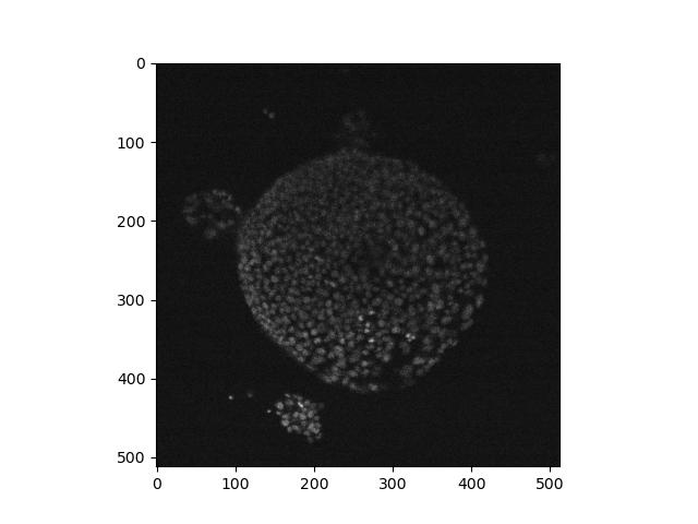
As discussed above in exercise 4, it may be difficult to distinguish a time series from a Z axis. You may also notice that here the X/Y axes are the latter two numbers, but in other examples above, the X/Y axes were the first two. This demonstrates the diversity and general lack of consistency in image formatting, and how it’s usually a good idea to find out as much as you can about the image from documentation and metadata before processing it.
Altering the lookup table
Now that we’ve been able to open an image, we can start to explore it and display it in different ways.
The imshow() function can take extra arguments in
addition to the image to display. One of these is called
cmap, which can apply alternate lookup tables (a.k.a.
colour maps):
Skimage uses lookup tables from the plotting library matplotlib. A list of available tables can be obtained with:
Exercise 5: Lookup tables
Go back to the FluorescentCells_3channel.tif image. Display each of
its three channels side by side in a matplotlib figure, each in a
different colour using cmap=. Use the values in
matplotlib.colormaps to select a lookup table for each
one.
There will be many ways to do this (and many colour maps to choose from!), but here is one possible solution:
PYTHON
# you'll need to run this again if you overwrote your `image` variable
image = imread('data/FluorescentCells_3channel.tif')
plt.figure(figsize=(12, 6))

plt.subplot(1, 3, 1)
plt.imshow(image[:, :, 0], cmap='Blues')

plt.subplot(1, 3, 2)
plt.imshow(image[:, :, 1], cmap='Oranges')

plt.subplot(1, 3, 3)
plt.imshow(image[:, :, 2], cmap='YlOrBr')
Exercise 5: Lookup tables (continued)
Load hela-cells_rgb.tif and try displaying it with different lookup tables. What results do you get? Why might this be the case?
The resulting image will not look as expected, and in Jupyter the image will appear unchanged. In this case, since the lookup table is being ignored, this would imply that the pixel values do not represent light intensities but rather are explicitly encoded colour values - i.e. it’s an RGB image.
Other notes
Rearranging channels
You may find yourself in a situation where the arrangement of
dimensions in your image is incorrect for the processing you wish to
perform on it - maybe a function requires that an image be oriented in a
particular way. This is where it’s useful to be able to rearrange the
dimensions of an image. To do this, we can use Numpy’s
moveaxis function:
PYTHON
import numpy
image = imread('data/FluorescentCells_3channel.tif')
print(image.shape)
# returns: (800, 800, 3)
rearranged_image = numpy.moveaxis(image, -1, 0)
print(rearranged_image.shape)
# returns: (3, 800, 800)
print(image.shape)
# returns: (800, 800, 3)
We can see that calling moveaxis on an array gives us a
rearranged version of the array given to it - the channel axis that was
at the end is now at the front. However, we can see that the original
value of the image is unchanged. This is because by default,
moveaxis returns a rearranged copy of the
image.
The arguments supplied are:
- The image or array
- The current position of the dimension to move
- The position to move that dimension to
In this case, we are moving the dimension at position -1 (i.e. the one at the end) to position 0 (the start).
Pixel size
Pixels are an approximation of an object - knowing that something is 50 pixels long and 50 pixels wide doesn’t tell us anything about its actual size. To make any real-world measurements on the image, we need the image’s pixel size.
To get this, it is necessary to read the image’s metadata. For this we need a different library, imageio. There are a couple of different places we can look:
PYTHON
import imageio
meta = imageio.v3.immeta('data/FluorescentCells_3channel.tif')
props = imageio.v3.improps('data/FluorescentCells_3channel.tif')
print('meta:', meta)
print('props:', props)
immeta() gives us a dict summarising the image, and
improps gives an object with the property ‘spacing’.
However, there is no guarantee that wither of these will contain any
information on pixel size, and the BioimageBook notes that these
numbers can be misleading and require interpretation and
cross-checking.
Even if immeta() does return a key called ‘unit’, the
value may be returned as escaped Unicode:
This can be un-escaped with:
Here, this would indicate that the image is to be mesaured in
micrometres. Combining this with other information that may be
available, e.g. improps().spacing, will help you figure out
the pixel size.
- Common image formats can usually all be loaded in the same way with skimage
- Specialised proprietary formats may require specialised libraries
- Basic metrics of an image include histogram, shape and max/min pixel values
- These metrics can help tell us how the miage should be analysed
- Lookup tables can change how a single-channel image is rendered
- An RGB image contains 3 channels for red, green and blue
Content from Applying Filters
Last updated on 2025-03-21 | Edit this page
Overview
Questions
- How can I make it possible to isolate features in my images?
Objectives
- Apply mean and Gaussian filters to an image
- Select one of these filtered images to use for processing in subsequent chapters
Filters
Images often need to have noise removed in order for the results of further processing to be meaningful. There are many smoothing filters available, each with their own advantages depending on the situation and the image in question. Here are two to get started:
A mean filter will, for each pixel:
- Create a kernel of pixels around it, in a size/shape of the user’s choosing
- Take the mean of all pixels within this kernel
- Assign this new value to the pixel
The kernel in this case can be considered analogous to a 2-dimensional sliding window.
A Gaussian filter is similar to a mean filter, except that pixels near the centre of the kernel will have a greater effect on the result.
You can create a kernel with skimage:
There are other shapes of kernel that can be used, and are documented in the morphology section of the skimage docs.
Note that as of skimage 0.25.0, the square function has
been deprecated in favour of a new function, footprint_rectangle:
PYTHON
from skimage.morphology import footprint_rectangle
kernel = square((3, 3)) # also a 3x3 square kernelExercise 6: Applying filters
Look at the documentation pages for the mean and Gaussian filters above. Load a frame from the second channel of the test image skimage.data.cells3d:
Build a figure displaying this image in each of the following forms:
- original image
- mean filter using a 3x3 square kernel
- mean filter using a 9x9 square kernel
- Gaussian filter of sigma = 1
- Gaussian filter of sigma = 5
How do the different methods compare?
PYTHON
from skimage.data import cells3d
from skimage.filters import gaussian
from skimage.filters.rank import mean
from skimage.morphology.footprints import square

image = cells3d()[30, 1, :, :]
plt.figure(figsize=(10, 12))

plt.subplot(3, 2, 1)
plt.imshow(image)
plt.title('Original')

plt.subplot(3, 2, 2)
plt.imshow(mean(image, footprint=square(3)))
plt.title('3x3 mean filter')

plt.subplot(3, 2, 3)
plt.imshow(mean(image, footprint=square(9)))
plt.title('9x9 mean filter')

plt.subplot(3, 2, 4)
plt.imshow(gaussian(image, sigma=1))
plt.title('Gaussian blur, σ=1')

plt.subplot(3, 2, 5)
plt.imshow(gaussian(image, sigma=5))
plt.title('Gaussian blur, σ=5')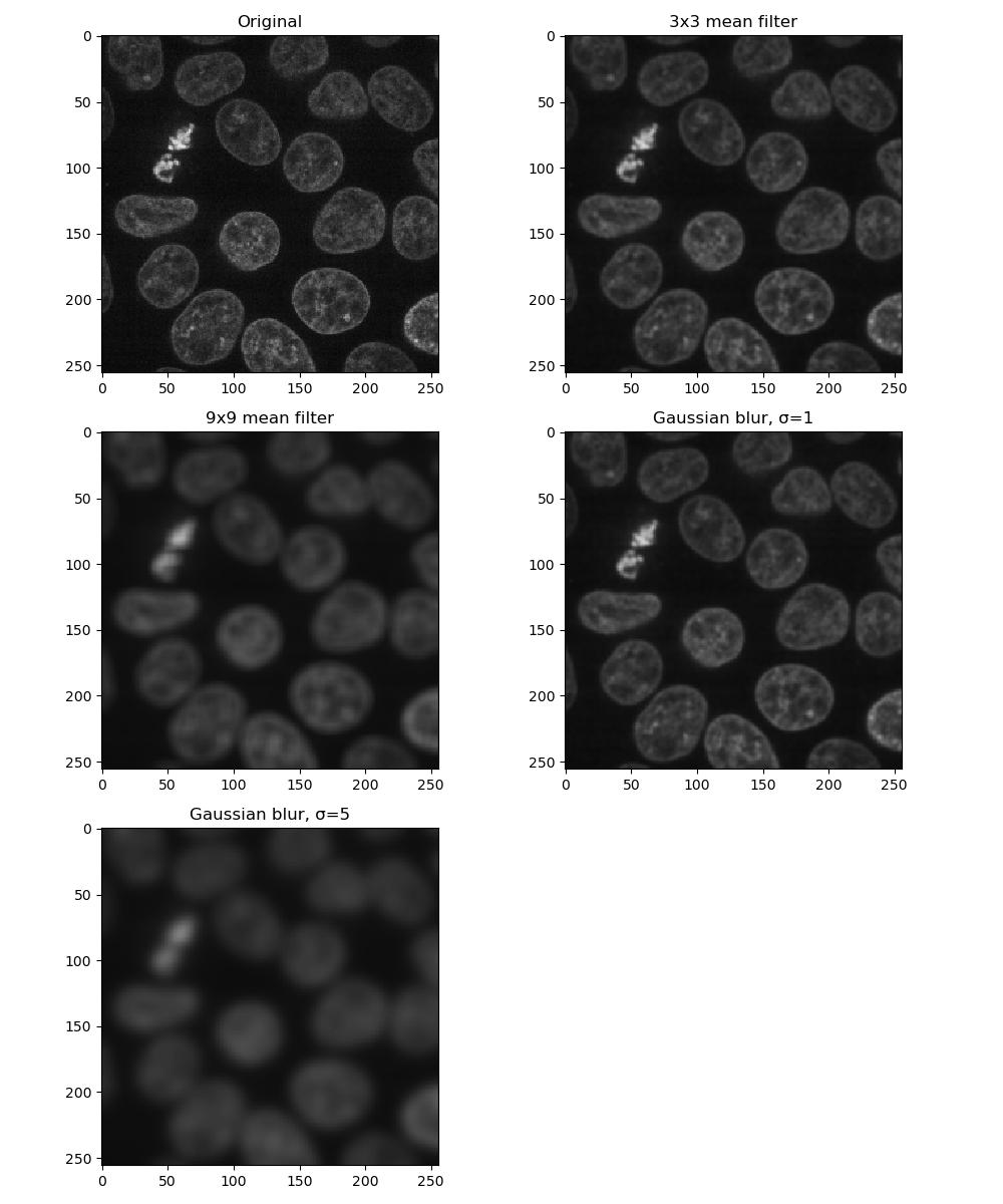
Larger kernels and sigma values will result in a greater smoothing effect and a more blurred image - as you can see, it is possible to over-blur the image.
Removing the background
Eventually we’re going to want to isolate the foreground from the background. In some images, this may be difficult especially if the two are not entirely distinct from each other, or if the background is not a uniform shade. In cases like this, a rolling ball algorithm can be applied. The rolling ball estimates the background intensity of an image by using the pixel values to translate the image into a height map, and then rolling a ball of a given radius across it. The rolling ball algorithm has been published and a figure from the publication describes how it works.
Exercise 7: Rolling ball background intensity
Look at the scikit-image documentation on the rolling ball filter. Load the example image skimage.data.coins and display:
- the original image
- image with a rolling ball of radius 100 applied
- image with a rolling ball of radius 50 applied
- the image with the radius=50 rolling ball subtracted from it
Compute time can be found using Python’s datetime library:
PYTHON
from skimage.data import coins
from skimage.restoration import rolling_ball

image = coins()
plt.figure(figsize=(10, 8))

plt.subplot(2, 2, 1)
plt.imshow(image, cmap='gray')
plt.title('Original')

plt.subplot(2, 2, 2)
rolling_ball_100 = rolling_ball(image, radius=100)
plt.imshow(rolling_ball_100, cmap='gray')
plt.title('Rolling ball, r=100')

plt.subplot(2, 2, 3)
rolling_ball_50 = rolling_ball(image, radius=50)
plt.imshow(rolling_ball_50, cmap='gray')
plt.title('Rolling ball, r=50')

plt.subplot(2, 2, 4)
plt.imshow(image - rolling_ball_50)
plt.title('Original - rolling ball r50')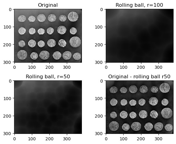
Dogs and logs
Difference of Gaussian (DoG) and Laplacian of Gaussian (LoG) are algorithms that build on the Gaussian filter.
In a Difference of Gaussian, two Gaussian filters are taken of the image, each with a different sigma value. The larger filter is then subtracted from the first to give an image where features are effectively highlighted by an area of high contrast.
In a Laplacian of Gaussian, a Gaussian-filtered image is supplied to a Laplace filter. This eliminates the need to manually select two sigma values as with Difference of Gaussian.
Exercise 8: Dogs and logs
Load a frame from the second channel of skimage.data.cells3d() again:
Display a figure of:
- The original image
- Image with a Difference of Gaussians applied with sigma values 2 and 4
- Image with a Laplacian of Gaussians applied. Note that the Laplace
filter linked above does not perform the Gaussian filter for you, so you
will need to pass the image through
gaussian()first.
PYTHON
from skimage.data import cells3d
from skimage.filters import gaussian, difference_of_gaussians, laplace

image = cells3d()[30, 1, :, :]
plt.figure(figsize=(10, 12))

plt.subplot(2, 2, 1)
plt.imshow(image)
plt.title('Original')

plt.subplot(2, 2, 2)
plt.imshow(difference_of_gaussians(image, 1, 2), cmap='gray')
plt.title('Difference of Gaussians')

plt.subplot(2, 2, 3)
plt.imshow(laplace(gaussian(image, sigma=2)), cmap='gray')
plt.title('Laplacian of Gaussian')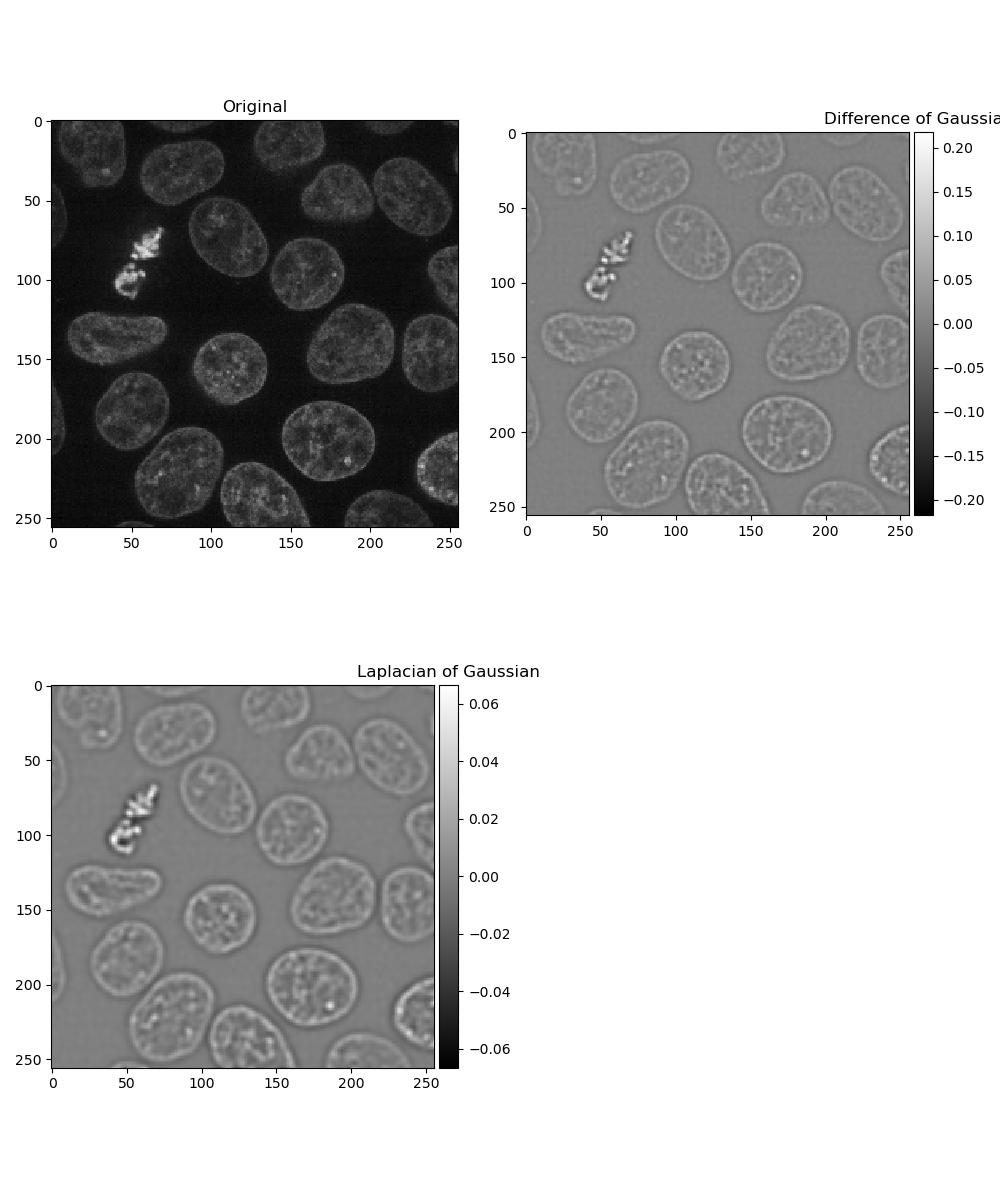
Exercise 9: Choosing a filter
Look at the images you produced in exercises 6 and 8, and select one to use in subsequent chapters for thresholding and segmentation!
- There are many ways of smoothing an image
- Different methods will perform better in different situations
Content from Thresholding and Segmentation
Last updated on 2025-03-24 | Edit this page
Overview
Questions
- How can I isolate features of interest in my image?
- How can I uniquely label features once I’ve found them?
Objectives
- Apply various thresholds an image
- Quantify features of interest in an image
- Demonstrate how to deal with edge cases like features stuck together
These exercises will make use of the image you decided to use in exercise 9.
Thresholding
Thresholding consists of converting an image into a binary form where each pixel value is either 0 or 1 depending on whether it exceeds a given threshold.
We can binarise an image with a given threshold by
applying the > operator to it. It’s common practice to
smooth the image first, e.g. with a Gaussian filter:
PYTHON
import matplotlib.pyplot as plt
from skimage.data import cells3d
from skimage.filters import gaussian

smoothed_image = gaussian(cells3d()[30, 1, :, :])
print(smoothed_image.min(), smoothed_image.max(), smoothed_image.dtype)

plt.subplot(1, 2, 1)
plt.imshow(smoothed_image, cmap='gray')
plt.title('Gaussian filter')

plt.subplot(1, 2, 2)
binary_image = smoothed_image > 0.12
plt.imshow(binary_image)
plt.title('Threshold > 0.12')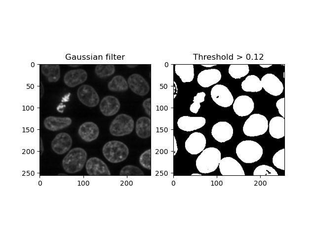
Applying a set number to an image as a threshold is simple, but it’s not ideal having to guess an appropriate threshold until we get a sensible one. Looking at the histogram helps, but still requires some manual interpretation and human subjectivity:
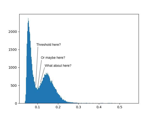
Fortunately, there are several algorithms for automatically determining an appropriate threshold based on the image’s histogram. Global thresholds work on the entire image, whereas local thresholds work on a window around each pixel - for the moment, we will only discuss global filters.
Exercise 10: Thresholds
Look at the skimage filter docs and find each of the following threshold algorithms:
- Otsu threshold
- Triangle threshold
Try running each of these algorithms on your smoothed image from exercise 9, and use the resulting threshold to binarise the image. How do the results differ?
We can display the two threshold algorithms in a figure:
PYTHON
from skimage.filters import threshold_otsu, threshold_triangle

plt.figure(figsize=(10, 8))

plt.subplot(1, 3, 1)
plt.imshow(smoothed_image)
plt.title('Gaussian filter')

# Otsu threshold
plt.subplot(1, 3, 2)
threshold = threshold_otsu(image)
plt.imshow(image > threshold)
plt.title('Otsu threshold')

# Triangle threshold
plt.subplot(1, 3, 3)
threshold = threshold_triangle(image)
plt.imshow(image > threshold)
plt.title('Triangle threshold')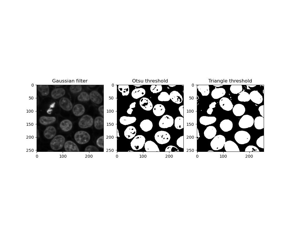
Which threshold performs better can depend on the image you have. Otsu thresholding is less sensitive so foreground objects are more likely to be incomplete or have holes in them, whereas triangle thresholding has a greater tendency for close foreground objects to become stuck together.
Cleaning up
Once we have a binary image, we may still need to clean it up further. There may still be extraneous pixels and other bits and pieces left around the regions of interest, or there may be holes in a shape that you need to be solid.
Exercise 11: Erosion, dilation, opening and closing
Look at the skimage morphology docs. Select one of your binary images from exercise 10 and apply each of the following algorithms to the image:
- Binary erosion
- Binary dilation
- Binary opening
- Binary closing
Note: each of the algorithms above will require a kernel or footprint. For each of these, use a disc-shaped kernel of radius 2:
PYTHON
from skimage.morphology import binary_erosion, binary_dilation, binary_opening, binary_closing
from skimage.morphology import disk
kernel = disk(2)
plt.figure(figsize=(8, 12))
# your binary image from exercise 10
plt.subplot(3, 2, 1)
plt.imshow(binary_image, cmap='gray')
plt.title('Binary image')
# erosion
plt.subplot(3, 2, 2)
plt.imshow(binary_erosion(binary_image, footprint=kernel), cmap='gray')
plt.title('Erosion')
# dilation
plt.subplot(3, 2, 3)
plt.imshow(binary_dilation(binary_image, footprint=kernel), cmap='gray')
plt.title('Dilation')
# opening
plt.subplot(3, 2, 4)
plt.imshow(binary_opening(binary_image, footprint=kernel), cmap='gray')
plt.title('Opening')
# closing
plt.subplot(3, 2, 5)
plt.imshow(binary_closing(binary_image, footprint=kernel), cmap='gray')
plt.title('Closing')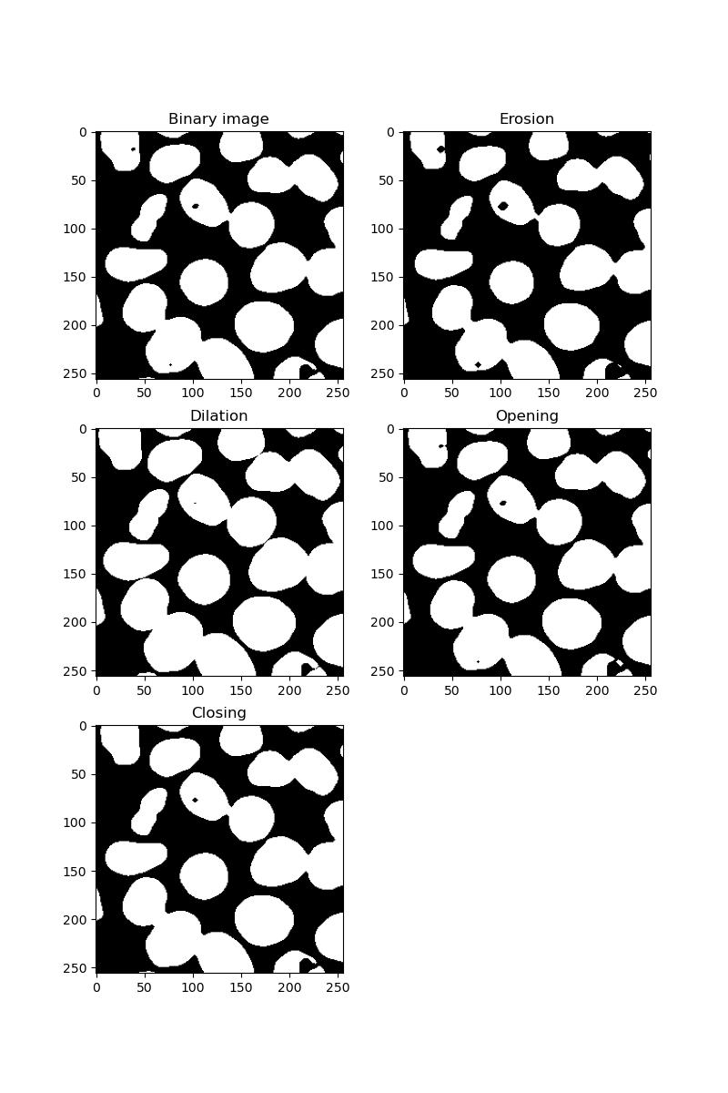
Eroding has the effect of shrinking all foreground features. Dilating has the opposite effect, potentially resulting in foreground features becoming stuck together.
Opening an image is an erosion followed by a dilation. If your image is grainy with many small artifacts, these will be removed.
Closing is the opposite - dilation followed by erosion. This will have the effect of filling in any holes in your foreground features.
If there are still holes in your binary image, there is also a function in scipy.ndimage that can fix this:
PYTHON
from scipy.ndimage import binary_fill_holes

fill_holes = binary_fill_holes(binary_image)
plt.imshow(fill_holes)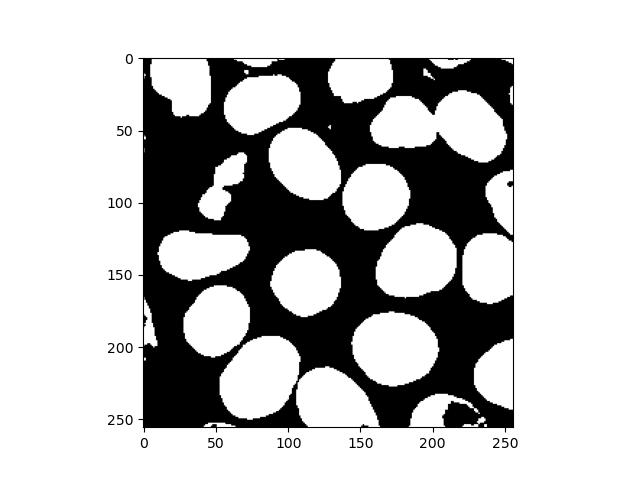
Labelling
In some situations, it may be necessary to distinguish between individual features, e.g. if counting cell nuclei. For this, it is necessary to isolate or label individual separated objects in the foreground:
PYTHON
from skimage.morphology import label

labels = label(fill_holes)
plt.imshow(labels, cmap='viridis')
plt.colorbar()
This will result in an image similar to the binary image supplied, but instead of just 1s, each feature will have a unique number assigned to all of its pixels. Displaying this with a colour scale will effectively colour-code each one:
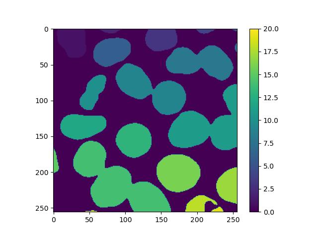
However, we can see that the process is not perfect, as nuclei that are stuck together have been marked as the same feature. In the exercises below, we will explore how to solve this.
Watershed transform
Several transforming or segmentation operations exist for solving situations like the one above with touching objects.
This transformation requires a few preparation steps. First, we need a distance transform of the binary image, where each foreground pixel’s value is its Euclidean distance to the background. skimage doesn’t have a function for this, but scipy does:
PYTHON
from scipy.ndimage import distance_transform_edt

dt = distance_transform_edt(fill_holes)
plt.imshow(dt)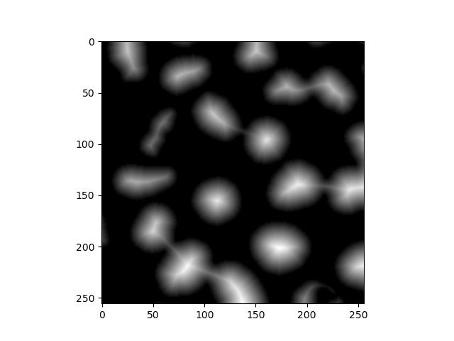
Next, we need the coordinates of all local maxima, i.e. locations that are furthest away from the background. This requires a kernel/footprint, which in this example is a square kernel of 7x7:
This gives us a list of coordinates, so we need to convert this back into an labelled image of maxima. This will be mostly blank with an individually labelled dot representing each one:
PYTHON
from numpy import zeros

mask = zeros(dt.shape, dtype=bool)  # create a blank image the same size as the original
mask[tuple(coords.T)] = True  # create a foreground pixel at each coordinate
markers = label(mask)  # uniquely label them
plt.imshow(markers, cmap='viridis')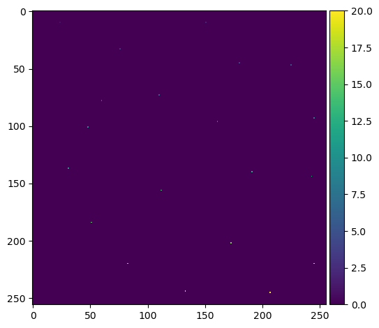
Note the .T to transpose the maxima coordinates.
At this point depending on your image, you may get clusters of peaks close together rather than one clean, distinct peak per feature. This is especially likely if your features are not circular. Applied to the final watershed step below, this will result in features being split when they shouldn’t be. This can be resolved in several ways:
Applying a larger footprint to peak_local_max
There are a few different ways to do this - all we need to do is create a kernel of a cerain shape and size, and pass it to peak_local_max:
PYTHON
# numpy
from numpy import ones
coords = peak_local_max(dt, footprint=ones((7,7)), labels=fill_holes)

# skimage < 0.25.0
coords = peak_local_max(dt, footprint=square(7), labels=fill_holes)

# skimage >= 0.25.0
coords = peak_local_max(dt, footprint=footprint_rectangle((7, 7)), labels=fill_holes)
Providing a min_distance argument to
peak_local_max
This will prevent the function from identifying peaks too close together:
Masked watershed
Now that we have identified some peaks, we can now put the distance transform together with the local peaks to do the transform:
PYTHON
from skimage.segmentation import watershed

watershed_transform = watershed(-dt, markers)
plt.imshow(watershed_transform, cmap='viridis')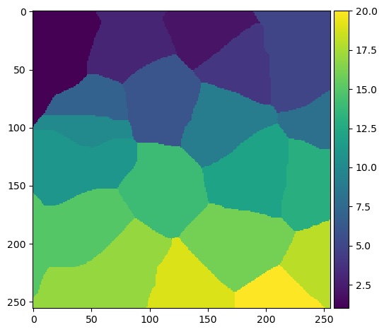
Note the - in front of the distance transform. This
effectively converts it from a map of peaks to a map of troughs. We need
to do this because of the way
watershed transforms work.
The result of the watershed transform above does not indicate the shape of the nuclei. Rather, the algorithm effectively decides which nucleus each pixel of the image most closely corresponds to. We can generate a more meaningful image by multiplying the watershed and the binary image together to create a masked watershed:
PYTHON
masked_watershed = watershed_transform * binary_image
plt.imshow(masked_watershed, cmap='viridis')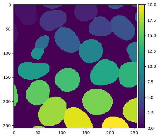
It’s also possible to do the last two steps in one by providing
mask=some_binary_image to
skimage.segmentation.watershed.
Exercise 12: Image segmentation
- Load up one of your cleaned up images from exercise 11 and run
skimage.morphology.labelon the foreground features - How many features did skimage find? (hint: try flattening your labelled image and printing the result to the screen)
- Perform a watershed transform on your binary image as above. Try displaying the result of each stage of the transform.
- How many features are identified now, after watershed transformation?
- Does the watershed transformation work perfectly?
Labelling applies a unique number to each feature. This means that if we apply thresholding and labelling to the image, we can flatten the result and cast it to a set to find all the unique label numbers present, and find the highest numbered label to get the number of features:
PYTHON
from skimage.data import cells3d
from skimage.filters import gaussian, threshold_otsu
from skimage.morphology import label

# whatever your chosen cleaned up image is
plt.subplot(1, 2, 1)
plt.imshow(binary_image)
plt.title('Cleaned up image')

# labelled
labels = label(binary_image)
plt.subplot(1, 2, 2)
plt.imshow(labels, cmap='viridis')
plt.title('Labelled')

flat = labels.flatten()
print(set(flat))
print('Features found:', max(flat))
However, we see from the intermediate images that multiple touching nuclei are treated as a single feature.
Here is an example of using distance and watershed transforms to segment touching objects:
PYTHON
from skimage.feature import peak_local_max
from skimage.segmentation import watershed
from scipy.ndimage import distance_transform_edt

dt = distance_transform_edt(binary_image)
plt.subplot(2, 2, 1)
plt.imshow(dt)
plt.title('Distance transform')

coords = peak_local_max(dt, min_distance=10, labels=binary_image)
mask = numpy.zeros(dt.shape, dtype=bool)
mask[tuple(coords.T)] = True
plt.subplot(2, 2, 2)
plt.imshow(mask, cmap='viridis')
plt.title('Markers')

markers = label(mask)
labels = watershed(-dt, markers, mask=binary_image)
plt.subplot(2, 2, 3)
plt.imshow(labels, cmap='viridis')
print('Features found:', max(labels.flatten()))
This will segment more correctly, however the accuracy of the process still depends on the inputs supplied. Irregular objects with holes in them will be harder to segment than even, solid, rounded shapes.
- Thresholding, labelling and feature isolation are all forms of segmentation
- Different thresholding algorithms can perform differently in different situations
- Quantitative image analysis often requires us to individually label features
- Processing such as watershed transforms can solve cases where features of interest are very close or stuck together
Content from Measurements
Last updated on 2025-03-21 | Edit this page
Overview
Questions
- How can I make useful measurements in my image?
Objectives
- Find the mean pixel intensity in each nucleus
- Find the area of each nucleus
Having isolated individual nuclei in the example image in the previous chapter, we can make some observations about the image features. The exercises here will require:
- Your masked watershed transformation from the previous chapter
- Your original smoothed image from exercise 9
Processing one nucleus at a time
Remember that each nucleus is labelled with a unique number, so we use masking to select a single nucleus. We can construct a binary mask from a labelled image using numpy’s where function:
PYTHON
from numpy import where

nucleus_1 = where(masked_watershed == 1, 1, 0)
nucleus_2 = where(masked_watershed == 2, 1, 0)
Here, each pixel will be set to either 1 or 0 depending on whether its value matches the label we’re looking for, effectively creating a binary mask for each nucleus.
Exercise 13: Quantifying intensities
For each labelled nucleus:
- Construct a binary mask matching the label number
- Use this to isolate the individual nucleus out of your
original smoothed image
- Hint: try looking at the
numpy.wheredocs to see the different ways it can be used.
- Hint: try looking at the
- Find the mean pixel value for the nucleus
First, we need to know how many features we’re looping over. We can get that from the numbers that the labelling process provides - if your labelled image contains the labels 1, 2 and 3, then you have 3 features.
Next, we need to generate a mask for that feature using
numpy.where, that will allow us to mask out the original
image - in this case, either a corresponding pixel value from the
original image or None. We can then take the result of
that, select all pixels that are not None and use
numpy.mean.
PYTHON
plt.figure(figsize=(12, 8))
labels = sorted(set(masked_watershed.flatten()))

for i in labels[:6]:  # just showing the first 6
    mask = numpy.where(masked_watershed == i, 1, 0)
    nucleus = numpy.where(mask == 1, image, 0)
    plt.subplot(2, 3, i + 1)  # subplot counts from 1 rather than 0
    plt.imshow(nucleus)
    pixels = [p for p in nucleus.flatten() if p]  # remove the background pixels
    print('Feature ' + str(i) + ':', numpy.mean(pixels))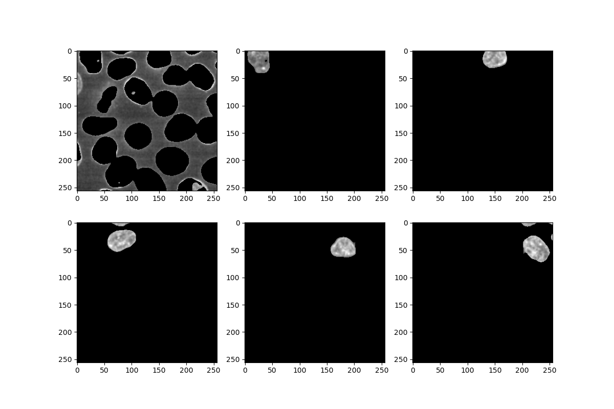
A few notes:
- Note how the first feature labelled as
0corresponds to the background - Remember that in
subplot, we need to offset the subplot number by +1, since it counts from 1 - In the first
numpy.whereabove, we supply two single numbers, 1 and 0, giving us a binary mask. In the next one, we provide an n-dimensional array instead, causing it to instead select the value of the corresponding pixel.
- Binary multiplication and
numpy.whereare powerful ways of combining images and masks - The numbers assigned during labelling can be used to select and process one feature at a time
Content from Introduction to Napari
Last updated on 2025-03-18 | Edit this page
Overview
Questions
- How can I view images and metadata in Napari?
Objectives
- Open and explore some images and compare the process of doing the same process in Python
Starting Napari
With Napari installed and its Conda environment active, run:
This will start up Napari in a new window. This may take about a minute, especially the first time.
Looking around
In the ‘File’ menu, go to ‘Open Sample -> napari builtins -> Cells (3D+2Ch)’. Looking at the sidebar, Napari has opened two layers - ‘membrane’ and ‘nuclei’. At the top of the sidebar there are options for displaying layers in different colours and opacity, and the eye symbol on the layer can be checked or unchecked to show/hide it:
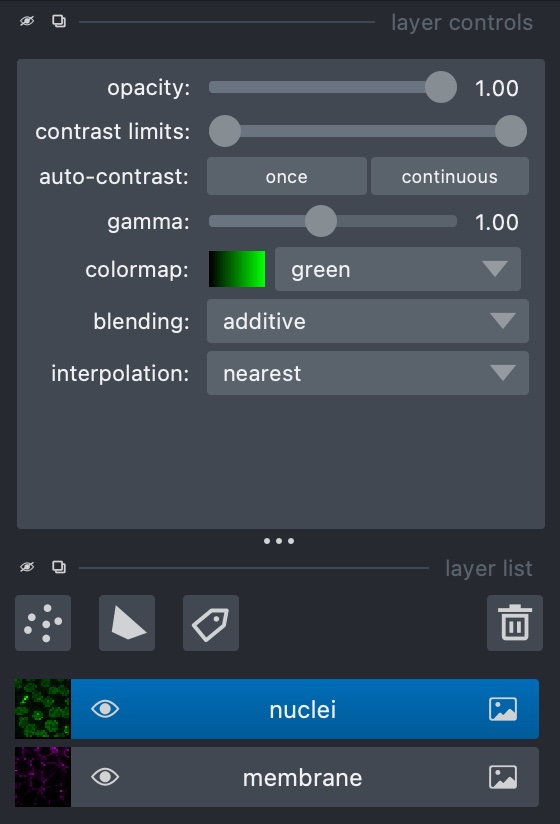
Napari uses layers to represent each stage of processing an image - we run tools to create new processed layers based off of a previous one. In this example, the image consists of two channels, each of which has been loaded as a layer.
In the case of z-stack or time series images such as this one, there is also a slider at the bottom for scrolling through the layers.
Exercise 14: Napari tools
With ‘Cells (3D + 2Ch)’ open, go to ‘Tools -> Filtering / Noise Removal’ and look at the options available. What are these options? What happens if you select one and try running it on a layer?
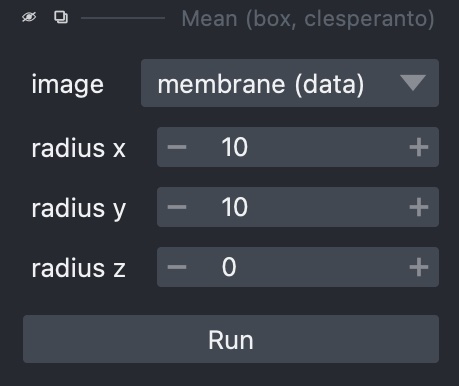
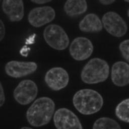
The options here consist of smoothing filters, several of which will be familiar from previous chapters. In some cases there are multiple versions of a filter (e.g. there are three Gaussian filters), each of which uses a different Python library.
Selecting one of these gives a sidebar letting us choose how to run it, including which layer to use, plus any extra parameters it may take, such as sigma values for Gaussian filters:
Loading real-world images
The example images work nicely with Napari, but sometimes it may be more difficult to coax Napari into loading an image correctly. In ‘File’, select ‘Open File(s)…’ and load up FluorescentCells_3channel.tif. Doing this, we find the results aren’t quite what we expect - the three channels have been loaded as if they’re a z-stack.
Fortunately, Napari includes a Python console that gives us very
fine-grained control of the user interface, and will let us load this
image correctly. In the bottom left, use the ’>_’ button to open a
terminal. This activates a Python session where Napari is represented as
an object called viewer:

- All the loaded layers are in a list called
viewer.layers - Within a layer, the image data is an attribute called
data
In this console, we can create new layers with
viewer.add_image. First, let’s look at the image’s
shape:
PYTHON
from skimage.io import imread
image = imread('path/to/FluorescentCells_3channel.tif')
image.shape
# returns: (512, 512, 3)
From this, we can see that the colour channels are the third axis. Using this, We can now load each channel as a new layer:
PYTHON
viewer.add_image(image[:, :, 0], name='FluorescentCells_ch0', colormap='red')
viewer.add_image(image[:, :, 1], name='FluorescentCells_ch1', colormap='green', blending='additive')
viewer.add_image(image[:, :, 2], name='FluorescentCells_ch2', colormap='blue', blending='additive')
The blending='additive' option prevents layers on top
from obscuring layers below it so that we can view multiple layers at
once. We also use colormap to colour the layers so we can
distinguish them from each other.
viewer.add_image is also able to load all these layers
in one if we tell it which axis represents the colour channels:
Exercise 15: Real world images
- Go to ‘File’ -> ‘Open File(s)…’ and load the image ‘confocal-series_zstack.tif’. How does it look? Can you view each channel simultaneously?
- Now try loading the same image in the console as above, looking at
the image’s shape and passing the channel axis to
viewer_add_image. axis looks like the channels. How has the fourth axis been represented?
Loading the image from the menu, we can see some results but it’s all in one layer and the channel axis is represented as a slider, meaning we can’t view the two at the same time.
As an alternative, we can load the image in the Python console:
PYTHON
image = imread('path/to/confocal-series_zstack.tif')
image.shape
# returns: (25, 2, 400, 400)
The second number, i.e. image.shape[1] looks like the
channel axis. We can then provide this when loading the image:
Napari will load the image as two coloured layers, with the Z axis represented via the slider at the bottom.
Exercise 16: Image segmentation in the Napari console
This exercise will put together everything that has been covered in previous chapters, and apply the same steps in the Napari console.
Look at the ‘nuclei’ layer of ‘Cells (3D + 2Ch)’. In the Python console, try doing the same smoothing, binarisation, segmentation and labelling that you performed throughout exercises 6-12, except displaying each step as a new layer in the Napari viewer.
Remember that instead of matplotlib.pyplot.imshow(),
you’ll need to use viewer.add_image()
PYTHON
import skimage

image = skimage.data.cells3d()
image.shape
# returns: (60, 2, 256, 256)

frame = image[30, 1, :, :]
smoothed_image = skimage.filters.gaussian(frame, sigma=1)
viewer.add_image(smoothed_image, name='smoothed')

threshold = skimage.filters.threshold_otsu(smoothed_image)
binary_image = smoothed_image > threshold
viewer.add_image(binary_image, name='Otsu threshold')

import scipy.ndimage
fill_holes = scipy.ndimage.binary_fill_holes(binary_image)
viewer.add_image(fill_holes, name='fill_holes')

distance_transform = scipy.ndimage.distance_transform_edt(fill_holes)
viewer.add_image(distance_transform, name='distance_transform')

coords = skimage.feature.peak_local_max(skimage.filters.gaussian(distance_transform, sigma=4), labels=fill_holes)

import numpy
mask = numpy.zeros(distance_transform.shape, dtype=bool)
mask[tuple(coords.T)] = True
markers = skimage.morphology.label(mask)
viewer.add_image(markers, name='peaks')

watershed_transform = skimage.segmentation.watershed(-distance_transform, markers)
viewer.add_image(watershed_transform, name='watershed')

masked_watershed = watershed_transform * fill_holes
viewer.add_image(masked_watershed, name='masked_watershed')
Image segmentation with Napari tools
Aside from running analyses in the Python console, Napari has a variety of processing steps that can be browsed under ‘Tools’.
For example, we can go to ‘Open Sample’ -> ‘napari builtins’ and -> ‘Binary Blobs’. Browse the tools available and run:
- Otsu threshold
- Split touching objects (nsbatwm). Try experimenting with different sigma values until you get some good cell separations.
- Connected component labelling (scikit-image, nsbatwm)
Note: The Otsu threshold shouldn’t be required since the test image is already a binary, but the ‘Split touching objects’ Napari tool isn’t able to recognise the original as a binary image. This is because Napari expects the values to be 0/1, whereas the test image uses the values True/False. Thresholding the image again converts it to the right type.
Exercise 17: Exporting code
This exercise will see how the processing that we have built up with Napari tools can be exported back to Python code that we can then check into version control and integrate into a workflow to help automate the processing of many images.
Under ‘Plugins’, open the Napari Assistant and find the ‘Export Python code’ tool. Use this to generate a Python script that will perform the processing that you just performed above on the Binary Blobs image. Does the script look usable immediately without modification?
There are several options to export in different ways, including to a Jupyter notebook. The simplest way is probably to copy to clipboard - this can be pasted into a text editor or IDE:
PYTHON
from skimage.io import imread
import napari_segment_blobs_and_things_with_membranes as nsbatwm  # version 0.3.6
import napari
if 'viewer' not in globals():
    viewer = napari.Viewer()

image0_bb = viewer.layers['binary_blobs'].data

# threshold otsu

image1_to = nsbatwm.threshold_otsu(image0_bb)
viewer.add_labels(image1_to, name='Result of threshold_otsu')

# split touching objects

image2_sto = nsbatwm.split_touching_objects(image1_to, 5.6)
viewer.add_labels(image2_sto, name='Result of split_touching_objects')

# connected component labeling

image3_ccl = nsbatwm.connected_component_labeling(image2_sto, False)
viewer.add_labels(image3_ccl, name='Result of connected_component_labeling')
Looking at it, we can see that it’s not immediately usable but it’s pretty close. Exported scripts do not make any reference to what image file was loaded, and there is no code at the end for writing the resuults to a file, so this is what you would need to add to get it to produce tangible output.
- Napari works with layers, each of which represents an image channel
- Napari doesn’t always know how to load a multi-channel image from the GUI
- We can use the Python console to perform custom operations that can’t be done in the GUI
- Most operations we performed earlier in Python can also be done in Napari, either graphically or in the terminal
