Applying Filters
Last updated on 2025-03-21 | Edit this page
Overview
Questions
- How can I make it possible to isolate features in my images?
Objectives
- Apply mean and Gaussian filters to an image
- Select one of these filtered images to use for processing in subsequent chapters
Filters
Images often need to have noise removed in order for the results of further processing to be meaningful. There are many smoothing filters available, each with their own advantages depending on the situation and the image in question. Here are two to get started:
A mean filter will, for each pixel:
- Create a kernel of pixels around it, in a size/shape of the user’s choosing
- Take the mean of all pixels within this kernel
- Assign this new value to the pixel
The kernel in this case can be considered analogous to a 2-dimensional sliding window.
A Gaussian filter is similar to a mean filter, except that pixels near the centre of the kernel will have a greater effect on the result.
You can create a kernel with skimage:
There are other shapes of kernel that can be used, and are documented in the morphology section of the skimage docs.
Note that as of skimage 0.25.0, the square function has
been deprecated in favour of a new function, footprint_rectangle:
PYTHON
from skimage.morphology import footprint_rectangle
kernel = square((3, 3)) # also a 3x3 square kernelExercise 6: Applying filters
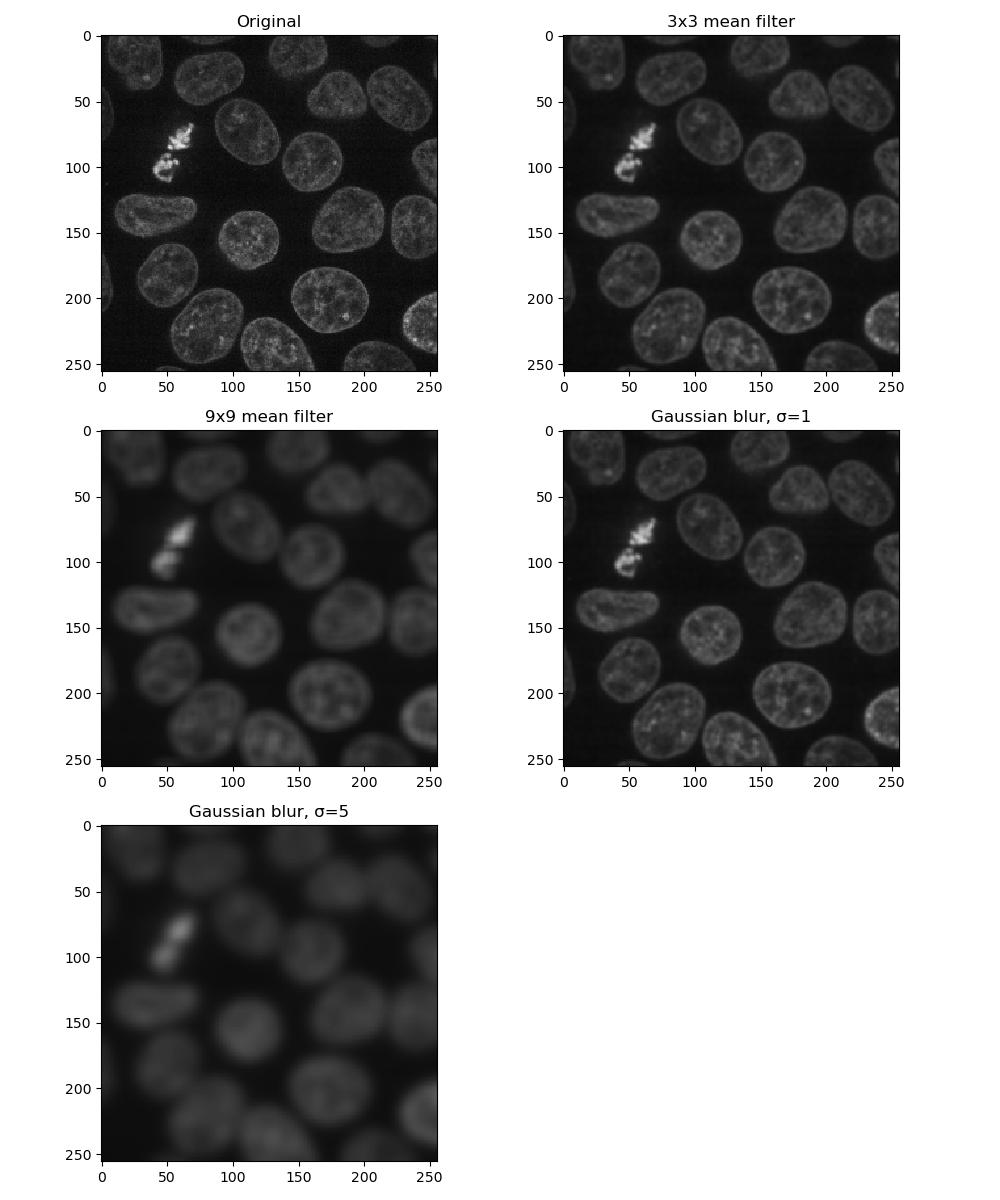
Look at the documentation pages for the mean and Gaussian filters above. Load a frame from the second channel of the test image skimage.data.cells3d:
Build a figure displaying this image in each of the following forms:
- original image
- mean filter using a 3x3 square kernel
- mean filter using a 9x9 square kernel
- Gaussian filter of sigma = 1
- Gaussian filter of sigma = 5
How do the different methods compare?
PYTHON
from skimage.data import cells3d
from skimage.filters import gaussian
from skimage.filters.rank import mean
from skimage.morphology.footprints import square

image = cells3d()[30, 1, :, :]
plt.figure(figsize=(10, 12))

plt.subplot(3, 2, 1)
plt.imshow(image)
plt.title('Original')

plt.subplot(3, 2, 2)
plt.imshow(mean(image, footprint=square(3)))
plt.title('3x3 mean filter')

plt.subplot(3, 2, 3)
plt.imshow(mean(image, footprint=square(9)))
plt.title('9x9 mean filter')

plt.subplot(3, 2, 4)
plt.imshow(gaussian(image, sigma=1))
plt.title('Gaussian blur, σ=1')

plt.subplot(3, 2, 5)
plt.imshow(gaussian(image, sigma=5))
plt.title('Gaussian blur, σ=5')
Larger kernels and sigma values will result in a greater smoothing effect and a more blurred image - as you can see, it is possible to over-blur the image.
Removing the background
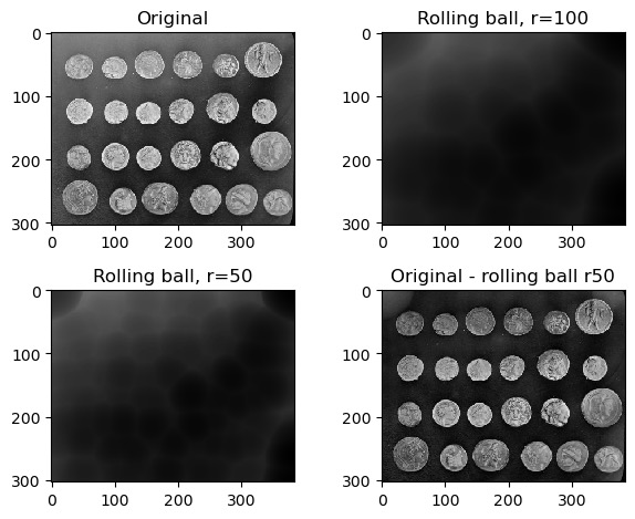
Eventually we’re going to want to isolate the foreground from the background. In some images, this may be difficult especially if the two are not entirely distinct from each other, or if the background is not a uniform shade. In cases like this, a rolling ball algorithm can be applied. The rolling ball estimates the background intensity of an image by using the pixel values to translate the image into a height map, and then rolling a ball of a given radius across it. The rolling ball algorithm has been published and a figure from the publication describes how it works.
Exercise 7: Rolling ball background intensity
Look at the scikit-image documentation on the rolling ball filter. Load the example image skimage.data.coins and display:
- the original image
- image with a rolling ball of radius 100 applied
- image with a rolling ball of radius 50 applied
- the image with the radius=50 rolling ball subtracted from it
Compute time can be found using Python’s datetime library:
PYTHON
from skimage.data import coins
from skimage.restoration import rolling_ball

image = coins()
plt.figure(figsize=(10, 8))

plt.subplot(2, 2, 1)
plt.imshow(image, cmap='gray')
plt.title('Original')

plt.subplot(2, 2, 2)
rolling_ball_100 = rolling_ball(image, radius=100)
plt.imshow(rolling_ball_100, cmap='gray')
plt.title('Rolling ball, r=100')

plt.subplot(2, 2, 3)
rolling_ball_50 = rolling_ball(image, radius=50)
plt.imshow(rolling_ball_50, cmap='gray')
plt.title('Rolling ball, r=50')

plt.subplot(2, 2, 4)
plt.imshow(image - rolling_ball_50)
plt.title('Original - rolling ball r50')
Dogs and logs
Difference of Gaussian (DoG) and Laplacian of Gaussian (LoG) are algorithms that build on the Gaussian filter.
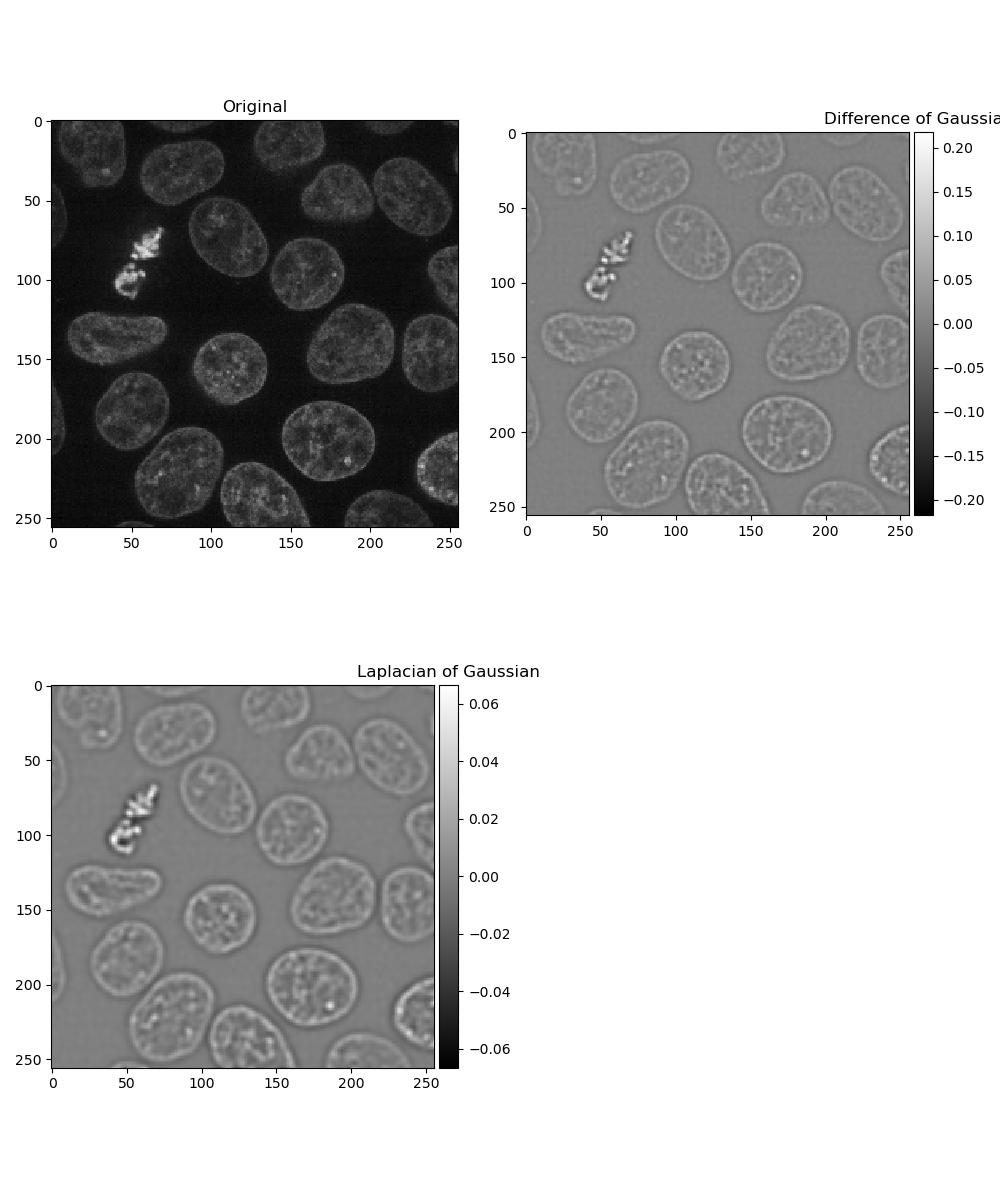
In a Difference of Gaussian, two Gaussian filters are taken of the image, each with a different sigma value. The larger filter is then subtracted from the first to give an image where features are effectively highlighted by an area of high contrast.
In a Laplacian of Gaussian, a Gaussian-filtered image is supplied to a Laplace filter. This eliminates the need to manually select two sigma values as with Difference of Gaussian.
Exercise 8: Dogs and logs
Load a frame from the second channel of skimage.data.cells3d() again:
Display a figure of:
- The original image
- Image with a Difference of Gaussians applied with sigma values 2 and 4
- Image with a Laplacian of Gaussians applied. Note that the Laplace
filter linked above does not perform the Gaussian filter for you, so you
will need to pass the image through
gaussian()first.
PYTHON
from skimage.data import cells3d
from skimage.filters import gaussian, difference_of_gaussians, laplace

image = cells3d()[30, 1, :, :]
plt.figure(figsize=(10, 12))

plt.subplot(2, 2, 1)
plt.imshow(image)
plt.title('Original')

plt.subplot(2, 2, 2)
plt.imshow(difference_of_gaussians(image, 1, 2), cmap='gray')
plt.title('Difference of Gaussians')

plt.subplot(2, 2, 3)
plt.imshow(laplace(gaussian(image, sigma=2)), cmap='gray')
plt.title('Laplacian of Gaussian')
Exercise 9: Choosing a filter
Look at the images you produced in exercises 6 and 8, and select one to use in subsequent chapters for thresholding and segmentation!
- There are many ways of smoothing an image
- Different methods will perform better in different situations
