Thresholding and Segmentation

Overview

Questions

• How can I isolate features of interest in my image?
• How can I uniquely label features once I’ve found them?

Objectives

• Apply various thresholds an image
• Quantify features of interest in an image
• Demonstrate how to deal with edge cases like features stuck together

These exercises will make use of the image you decided to use in exercise 9.

Thresholding

---

Thresholding consists of converting an image into a binary form where each pixel value is either 0 or 1 depending on whether it exceeds a given threshold.

We can binarise an image with a given threshold by applying the > operator to it. It’s common practice to smooth the image first, e.g. with a Gaussian filter:

PYTHON

import matplotlib.pyplot as plt
from skimage.data import cells3d
from skimage.filters import gaussian

smoothed_image = gaussian(cells3d()[30, 1, :, :])
print(smoothed_image.min(), smoothed_image.max(), smoothed_image.dtype)

plt.subplot(1, 2, 1)
plt.imshow(smoothed_image, cmap='gray')
plt.title('Gaussian filter')

plt.subplot(1, 2, 2)
binary_image = smoothed_image > 0.12
plt.imshow(binary_image)
plt.title('Threshold > 0.12')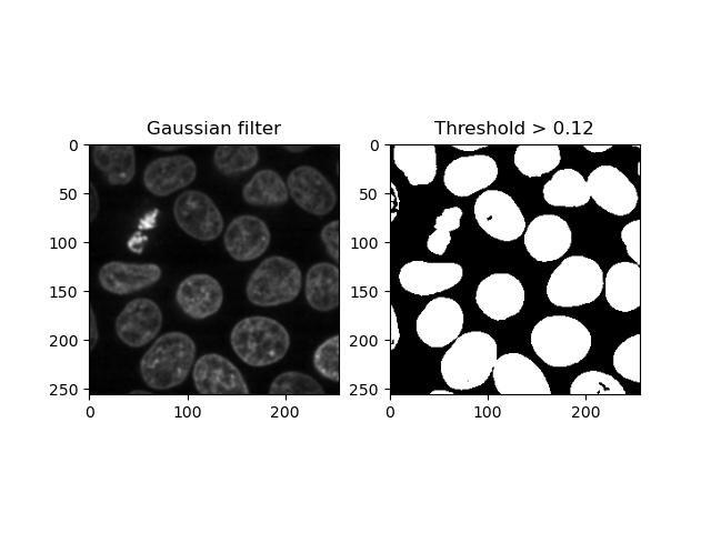

Applying a set number to an image as a threshold is simple, but it’s not ideal having to guess an appropriate threshold until we get a sensible one. Looking at the histogram helps, but still requires some manual interpretation and human subjectivity:

PYTHON

plt.hist(image.flatten(), bins=256)

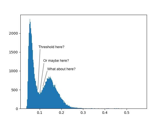
Fortunately, there are several algorithms for automatically determining an appropriate threshold based on the image’s histogram. Global thresholds work on the entire image, whereas local thresholds work on a window around each pixel - for the moment, we will only discuss global filters.

Exercise 10: Thresholds

Look at the skimage filter docs and find each of the following threshold algorithms:

• Otsu threshold
• Triangle threshold

Try running each of these algorithms on your smoothed image from exercise 9, and use the resulting threshold to binarise the image. How do the results differ?

Show me the solution

We can display the two threshold algorithms in a figure:

PYTHON

from skimage.filters import threshold_otsu, threshold_triangle

plt.figure(figsize=(10, 8))

plt.subplot(1, 3, 1)
plt.imshow(smoothed_image)
plt.title('Gaussian filter')

# Otsu threshold
plt.subplot(1, 3, 2)
threshold = threshold_otsu(image)
plt.imshow(image > threshold)
plt.title('Otsu threshold')

# Triangle threshold
plt.subplot(1, 3, 3)
threshold = threshold_triangle(image)
plt.imshow(image > threshold)
plt.title('Triangle threshold')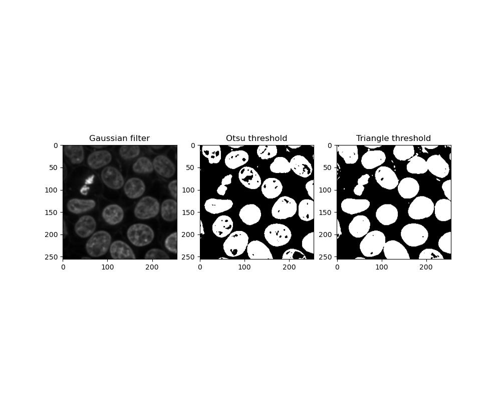

Which threshold performs better can depend on the image you have. Otsu thresholding is less sensitive so foreground objects are more likely to be incomplete or have holes in them, whereas triangle thresholding has a greater tendency for close foreground objects to become stuck together.

Cleaning up

---

Once we have a binary image, we may still need to clean it up further. There may still be extraneous pixels and other bits and pieces left around the regions of interest, or there may be holes in a shape that you need to be solid.

Exercise 11: Erosion, dilation, opening and closing

Look at the skimage morphology docs. Select one of your binary images from exercise 10 and apply each of the following algorithms to the image:

• Binary erosion
• Binary dilation
• Binary opening
• Binary closing

Note: each of the algorithms above will require a kernel or footprint. For each of these, use a disc-shaped kernel of radius 2:

PYTHON

from skimage.morphology import disk
kernel = disk(2)

Show me the solution

PYTHON

from skimage.morphology import binary_erosion, binary_dilation, binary_opening, binary_closing
from skimage.morphology import disk

kernel = disk(2)
plt.figure(figsize=(8, 12))

# your binary image from exercise 10
plt.subplot(3, 2, 1)
plt.imshow(binary_image, cmap='gray')
plt.title('Binary image')

# erosion
plt.subplot(3, 2, 2)
plt.imshow(binary_erosion(binary_image, footprint=kernel), cmap='gray')
plt.title('Erosion')

# dilation
plt.subplot(3, 2, 3)
plt.imshow(binary_dilation(binary_image, footprint=kernel), cmap='gray')
plt.title('Dilation')

# opening
plt.subplot(3, 2, 4)
plt.imshow(binary_opening(binary_image, footprint=kernel), cmap='gray')
plt.title('Opening')

# closing
plt.subplot(3, 2, 5)
plt.imshow(binary_closing(binary_image, footprint=kernel), cmap='gray')
plt.title('Closing')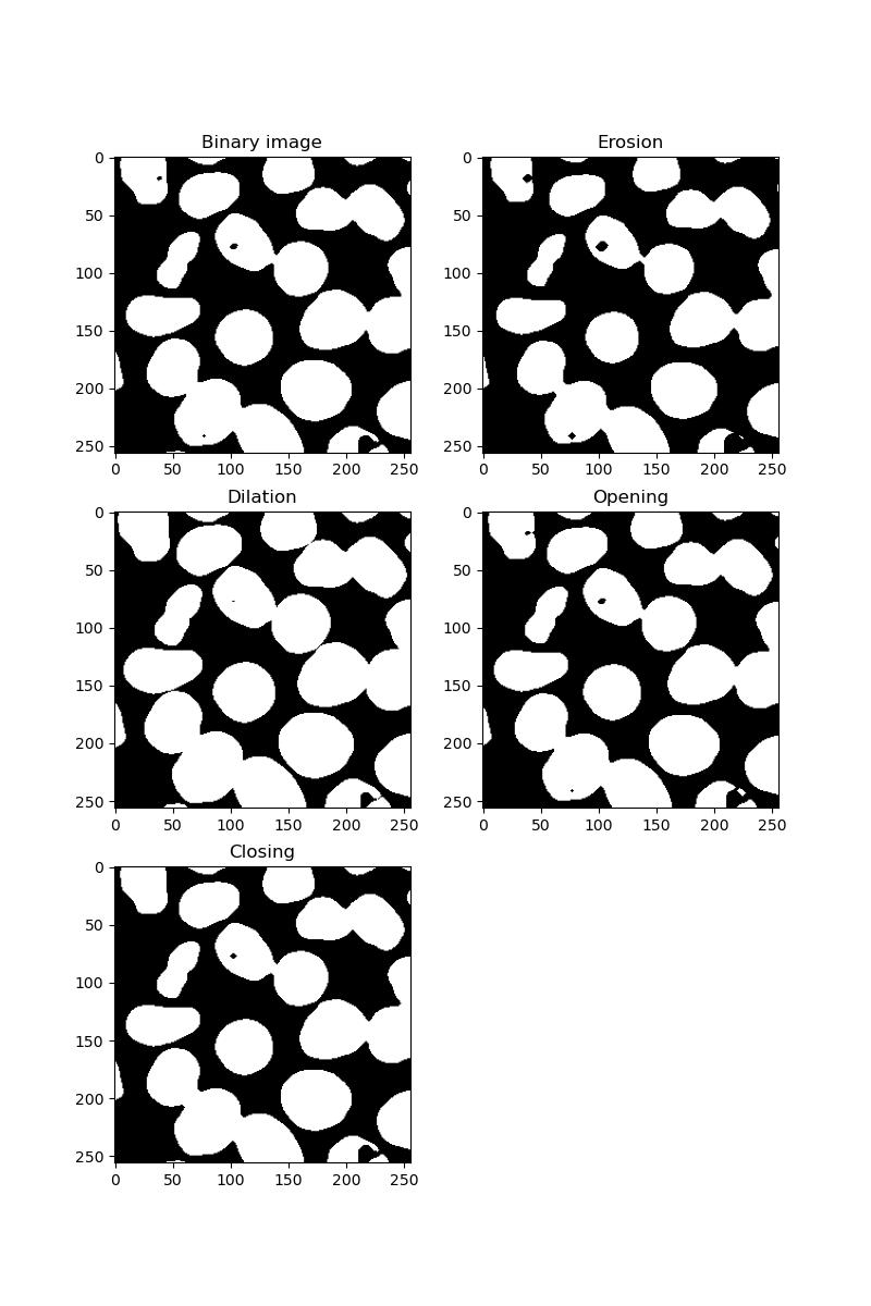

Eroding has the effect of shrinking all foreground features. Dilating has the opposite effect, potentially resulting in foreground features becoming stuck together.

Opening an image is an erosion followed by a dilation. If your image is grainy with many small artifacts, these will be removed.

Closing is the opposite - dilation followed by erosion. This will have the effect of filling in any holes in your foreground features.

If there are still holes in your binary image, there is also a function in scipy.ndimage that can fix this:

PYTHON

from scipy.ndimage import binary_fill_holes

fill_holes = binary_fill_holes(binary_image)
plt.imshow(fill_holes)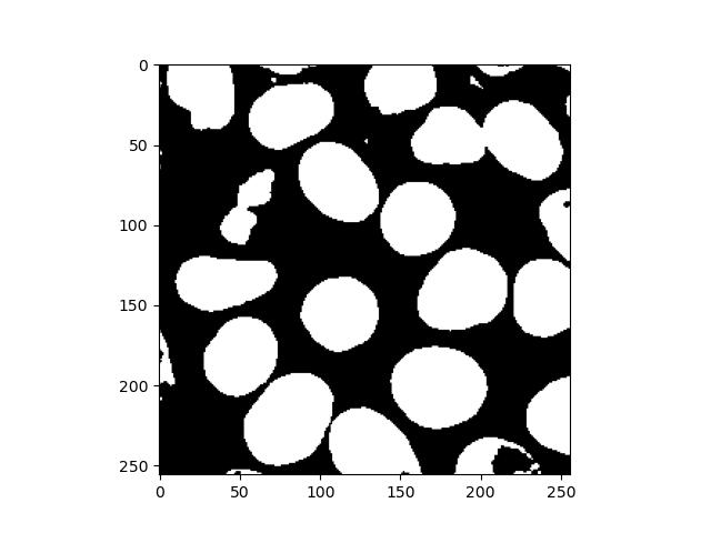

Labelling

---

In some situations, it may be necessary to distinguish between individual features, e.g. if counting cell nuclei. For this, it is necessary to isolate or label individual separated objects in the foreground:

PYTHON

from skimage.morphology import label

labels = label(fill_holes)
plt.imshow(labels, cmap='viridis')
plt.colorbar()

This will result in an image similar to the binary image supplied, but instead of just 1s, each feature will have a unique number assigned to all of its pixels. Displaying this with a colour scale will effectively colour-code each one:

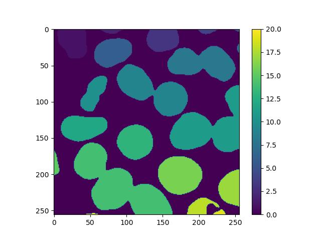
However, we can see that the process is not perfect, as nuclei that are stuck together have been marked as the same feature. In the exercises below, we will explore how to solve this.

Watershed transform

---

Several transforming or segmentation operations exist for solving situations like the one above with touching objects.

This transformation requires a few preparation steps. First, we need a distance transform of the binary image, where each foreground pixel’s value is its Euclidean distance to the background. skimage doesn’t have a function for this, but scipy does:

PYTHON

from scipy.ndimage import distance_transform_edt

dt = distance_transform_edt(fill_holes)
plt.imshow(dt)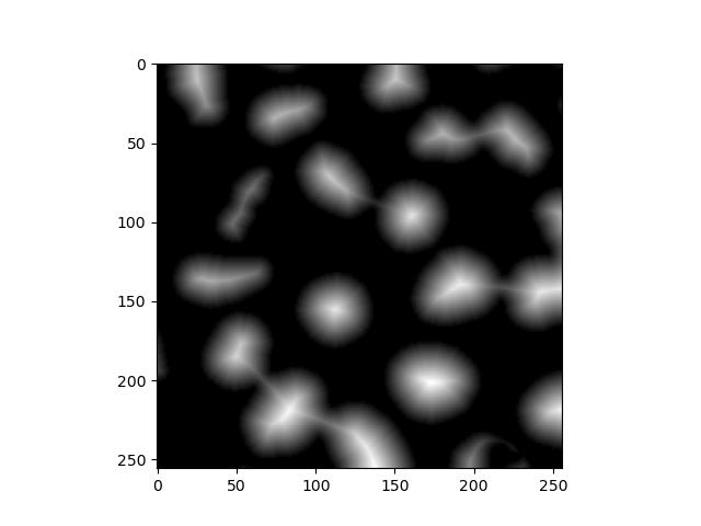

Next, we need the coordinates of all local maxima, i.e. locations that are furthest away from the background. This requires a kernel/footprint, which in this example is a square kernel of 7x7:

PYTHON

from skimage.feature import peak_local_max

coords = peak_local_max(dt, labels=fill_holes)

This gives us a list of coordinates, so we need to convert this back into an labelled image of maxima. This will be mostly blank with an individually labelled dot representing each one:

PYTHON

from numpy import zeros

mask = zeros(dt.shape, dtype=bool)  # create a blank image the same size as the original
mask[tuple(coords.T)] = True  # create a foreground pixel at each coordinate
markers = label(mask)  # uniquely label them
plt.imshow(markers, cmap='viridis')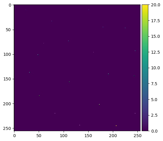

Note the .T to transpose the maxima coordinates.

At this point depending on your image, you may get clusters of peaks close together rather than one clean, distinct peak per feature. This is especially likely if your features are not circular. Applied to the final watershed step below, this will result in features being split when they shouldn’t be. This can be resolved in several ways:

Smoothing the distance transform first

PYTHON

coords = peak_local_max(gaussian(dt, sigma=4), labels=fill_holes)

Applying a larger footprint to peak_local_max

There are a few different ways to do this - all we need to do is create a kernel of a cerain shape and size, and pass it to peak_local_max:

PYTHON

# numpy
from numpy import ones
coords = peak_local_max(dt, footprint=ones((7,7)), labels=fill_holes)

# skimage < 0.25.0
coords = peak_local_max(dt, footprint=square(7), labels=fill_holes)

# skimage >= 0.25.0
coords = peak_local_max(dt, footprint=footprint_rectangle((7, 7)), labels=fill_holes)

Providing a min_distance argument to peak_local_max

This will prevent the function from identifying peaks too close together:

PYTHON

coords = peak_local_max(dt, min_distance=10, labels=fill_holes)

Masked watershed

Now that we have identified some peaks, we can now put the distance transform together with the local peaks to do the transform:

PYTHON

from skimage.segmentation import watershed

watershed_transform = watershed(-dt, markers)
plt.imshow(watershed_transform, cmap='viridis')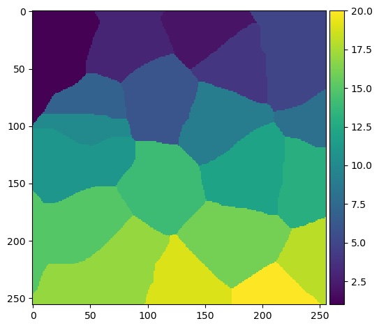

Note the - in front of the distance transform. This effectively converts it from a map of peaks to a map of troughs. We need to do this because of the way watershed transforms work.

The result of the watershed transform above does not indicate the shape of the nuclei. Rather, the algorithm effectively decides which nucleus each pixel of the image most closely corresponds to. We can generate a more meaningful image by multiplying the watershed and the binary image together to create a masked watershed:

PYTHON

masked_watershed = watershed_transform * binary_image
plt.imshow(masked_watershed, cmap='viridis')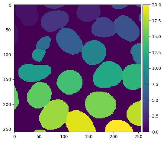

It’s also possible to do the last two steps in one by providing mask=some_binary_image to skimage.segmentation.watershed.

Exercise 12: Image segmentation

• Load up one of your cleaned up images from exercise 11 and run skimage.morphology.label on the foreground features
• How many features did skimage find? (hint: try flattening your labelled image and printing the result to the screen)
• Perform a watershed transform on your binary image as above. Try displaying the result of each stage of the transform.
• How many features are identified now, after watershed transformation?
• Does the watershed transformation work perfectly?

Show me the solution

Labelling applies a unique number to each feature. This means that if we apply thresholding and labelling to the image, we can flatten the result and cast it to a set to find all the unique label numbers present, and find the highest numbered label to get the number of features:

PYTHON

from skimage.data import cells3d
from skimage.filters import gaussian, threshold_otsu
from skimage.morphology import label

# whatever your chosen cleaned up image is
plt.subplot(1, 2, 1)
plt.imshow(binary_image)
plt.title('Cleaned up image')

# labelled
labels = label(binary_image)
plt.subplot(1, 2, 2)
plt.imshow(labels, cmap='viridis')
plt.title('Labelled')

flat = labels.flatten()
print(set(flat))
print('Features found:', max(flat))

However, we see from the intermediate images that multiple touching nuclei are treated as a single feature.

Here is an example of using distance and watershed transforms to segment touching objects:

PYTHON

from skimage.feature import peak_local_max
from skimage.segmentation import watershed
from scipy.ndimage import distance_transform_edt

dt = distance_transform_edt(binary_image)
plt.subplot(2, 2, 1)
plt.imshow(dt)
plt.title('Distance transform')

coords = peak_local_max(dt, min_distance=10, labels=binary_image)
mask = numpy.zeros(dt.shape, dtype=bool)
mask[tuple(coords.T)] = True
plt.subplot(2, 2, 2)
plt.imshow(mask, cmap='viridis')
plt.title('Markers')

markers = label(mask)
labels = watershed(-dt, markers, mask=binary_image)
plt.subplot(2, 2, 3)
plt.imshow(labels, cmap='viridis')
print('Features found:', max(labels.flatten()))

This will segment more correctly, however the accuracy of the process still depends on the inputs supplied. Irregular objects with holes in them will be harder to segment than even, solid, rounded shapes.

Key Points

• Thresholding, labelling and feature isolation are all forms of segmentation
• Different thresholding algorithms can perform differently in different situations
• Quantitative image analysis often requires us to individually label features
• Processing such as watershed transforms can solve cases where features of interest are very close or stuck together