Introduction to Napari
Last updated on 2025-03-18 | Edit this page
Estimated time: 90 minutes
Overview
Questions
- How can I view images and metadata in Napari?
Objectives
- Open and explore some images and compare the process of doing the same process in Python
Starting Napari
With Napari installed and its Conda environment active, run:
This will start up Napari in a new window. This may take about a minute, especially the first time.
Looking around
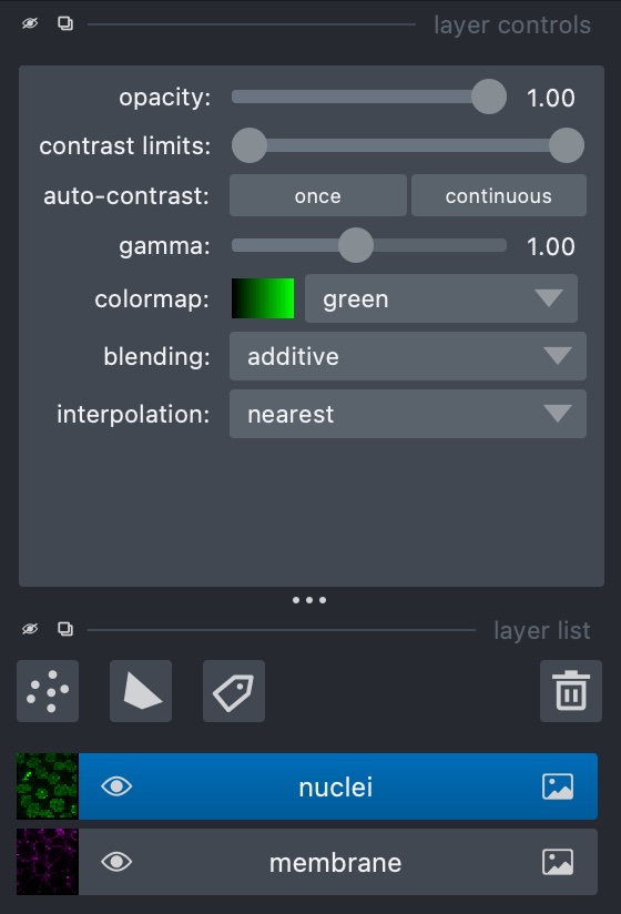
In the ‘File’ menu, go to ‘Open Sample -> napari builtins -> Cells (3D+2Ch)’. Looking at the sidebar, Napari has opened two layers - ‘membrane’ and ‘nuclei’. At the top of the sidebar there are options for displaying layers in different colours and opacity, and the eye symbol on the layer can be checked or unchecked to show/hide it:

Napari uses layers to represent each stage of processing an image - we run tools to create new processed layers based off of a previous one. In this example, the image consists of two channels, each of which has been loaded as a layer.
In the case of z-stack or time series images such as this one, there is also a slider at the bottom for scrolling through the layers.
Exercise 14: Napari tools
With ‘Cells (3D + 2Ch)’ open, go to ‘Tools -> Filtering / Noise Removal’ and look at the options available. What are these options? What happens if you select one and try running it on a layer?
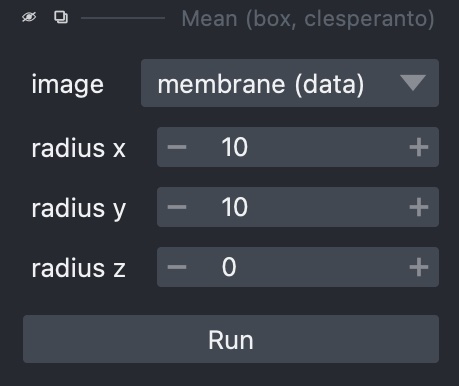
The options here consist of smoothing filters, several of which will be familiar from previous chapters. In some cases there are multiple versions of a filter (e.g. there are three Gaussian filters), each of which uses a different Python library.
Selecting one of these gives a sidebar letting us choose how to run it, including which layer to use, plus any extra parameters it may take, such as sigma values for Gaussian filters:


Loading real-world images
The example images work nicely with Napari, but sometimes it may be more difficult to coax Napari into loading an image correctly. In ‘File’, select ‘Open File(s)…’ and load up FluorescentCells_3channel.tif. Doing this, we find the results aren’t quite what we expect - the three channels have been loaded as if they’re a z-stack.
Fortunately, Napari includes a Python console that gives us very
fine-grained control of the user interface, and will let us load this
image correctly. In the bottom left, use the ’>_’ button to open a
terminal. This activates a Python session where Napari is represented as
an object called viewer:

- All the loaded layers are in a list called
viewer.layers - Within a layer, the image data is an attribute called
data
In this console, we can create new layers with
viewer.add_image. First, let’s look at the image’s
shape:
PYTHON
from skimage.io import imread
image = imread('path/to/FluorescentCells_3channel.tif')
image.shape
# returns: (512, 512, 3)
From this, we can see that the colour channels are the third axis. Using this, We can now load each channel as a new layer:
PYTHON
viewer.add_image(image[:, :, 0], name='FluorescentCells_ch0', colormap='red')
viewer.add_image(image[:, :, 1], name='FluorescentCells_ch1', colormap='green', blending='additive')
viewer.add_image(image[:, :, 2], name='FluorescentCells_ch2', colormap='blue', blending='additive')
The blending='additive' option prevents layers on top
from obscuring layers below it so that we can view multiple layers at
once. We also use colormap to colour the layers so we can
distinguish them from each other.
viewer.add_image is also able to load all these layers
in one if we tell it which axis represents the colour channels:
Exercise 15: Real world images
- Go to ‘File’ -> ‘Open File(s)…’ and load the image ‘confocal-series_zstack.tif’. How does it look? Can you view each channel simultaneously?
- Now try loading the same image in the console as above, looking at
the image’s shape and passing the channel axis to
viewer_add_image. axis looks like the channels. How has the fourth axis been represented?
Loading the image from the menu, we can see some results but it’s all in one layer and the channel axis is represented as a slider, meaning we can’t view the two at the same time.
As an alternative, we can load the image in the Python console:
PYTHON
image = imread('path/to/confocal-series_zstack.tif')
image.shape
# returns: (25, 2, 400, 400)
The second number, i.e. image.shape[1] looks like the
channel axis. We can then provide this when loading the image:
Napari will load the image as two coloured layers, with the Z axis represented via the slider at the bottom.
Exercise 16: Image segmentation in the Napari console
This exercise will put together everything that has been covered in previous chapters, and apply the same steps in the Napari console.
Look at the ‘nuclei’ layer of ‘Cells (3D + 2Ch)’. In the Python console, try doing the same smoothing, binarisation, segmentation and labelling that you performed throughout exercises 6-12, except displaying each step as a new layer in the Napari viewer.
Remember that instead of matplotlib.pyplot.imshow(),
you’ll need to use viewer.add_image()
PYTHON
import skimage

image = skimage.data.cells3d()
image.shape
# returns: (60, 2, 256, 256)

frame = image[30, 1, :, :]
smoothed_image = skimage.filters.gaussian(frame, sigma=1)
viewer.add_image(smoothed_image, name='smoothed')

threshold = skimage.filters.threshold_otsu(smoothed_image)
binary_image = smoothed_image > threshold
viewer.add_image(binary_image, name='Otsu threshold')

import scipy.ndimage
fill_holes = scipy.ndimage.binary_fill_holes(binary_image)
viewer.add_image(fill_holes, name='fill_holes')

distance_transform = scipy.ndimage.distance_transform_edt(fill_holes)
viewer.add_image(distance_transform, name='distance_transform')

coords = skimage.feature.peak_local_max(skimage.filters.gaussian(distance_transform, sigma=4), labels=fill_holes)

import numpy
mask = numpy.zeros(distance_transform.shape, dtype=bool)
mask[tuple(coords.T)] = True
markers = skimage.morphology.label(mask)
viewer.add_image(markers, name='peaks')

watershed_transform = skimage.segmentation.watershed(-distance_transform, markers)
viewer.add_image(watershed_transform, name='watershed')

masked_watershed = watershed_transform * fill_holes
viewer.add_image(masked_watershed, name='masked_watershed')
Image segmentation with Napari tools
Aside from running analyses in the Python console, Napari has a variety of processing steps that can be browsed under ‘Tools’.
For example, we can go to ‘Open Sample’ -> ‘napari builtins’ and -> ‘Binary Blobs’. Browse the tools available and run:
- Otsu threshold
- Split touching objects (nsbatwm). Try experimenting with different sigma values until you get some good cell separations.
- Connected component labelling (scikit-image, nsbatwm)
Note: The Otsu threshold shouldn’t be required since the test image is already a binary, but the ‘Split touching objects’ Napari tool isn’t able to recognise the original as a binary image. This is because Napari expects the values to be 0/1, whereas the test image uses the values True/False. Thresholding the image again converts it to the right type.
Exercise 17: Exporting code
This exercise will see how the processing that we have built up with Napari tools can be exported back to Python code that we can then check into version control and integrate into a workflow to help automate the processing of many images.
Under ‘Plugins’, open the Napari Assistant and find the ‘Export Python code’ tool. Use this to generate a Python script that will perform the processing that you just performed above on the Binary Blobs image. Does the script look usable immediately without modification?
There are several options to export in different ways, including to a Jupyter notebook. The simplest way is probably to copy to clipboard - this can be pasted into a text editor or IDE:
PYTHON
from skimage.io import imread
import napari_segment_blobs_and_things_with_membranes as nsbatwm  # version 0.3.6
import napari
if 'viewer' not in globals():
    viewer = napari.Viewer()

image0_bb = viewer.layers['binary_blobs'].data

# threshold otsu

image1_to = nsbatwm.threshold_otsu(image0_bb)
viewer.add_labels(image1_to, name='Result of threshold_otsu')

# split touching objects

image2_sto = nsbatwm.split_touching_objects(image1_to, 5.6)
viewer.add_labels(image2_sto, name='Result of split_touching_objects')

# connected component labeling

image3_ccl = nsbatwm.connected_component_labeling(image2_sto, False)
viewer.add_labels(image3_ccl, name='Result of connected_component_labeling')
Looking at it, we can see that it’s not immediately usable but it’s pretty close. Exported scripts do not make any reference to what image file was loaded, and there is no code at the end for writing the resuults to a file, so this is what you would need to add to get it to produce tangible output.
- Napari works with layers, each of which represents an image channel
- Napari doesn’t always know how to load a multi-channel image from the GUI
- We can use the Python console to perform custom operations that can’t be done in the GUI
- Most operations we performed earlier in Python can also be done in Napari, either graphically or in the terminal
