Opening and Checking an Image
Last updated on 2026-04-30 | Edit this page
Estimated time: 80 minutes
Overview
Questions
- How do I open an image file in Python for processing?
- How can I explore an image once it’s open?
Objectives
- Open an image with skimage
- Discuss how to open proprietary image formats
- Display an opened image to the screen
Opening an image
At its core, an image is a multidimensional array of numbers, and as
such can be opened by programs and libraries designed for working with
this kind of data. For Python, one such library is scikit-image. This
library provides a function called imread that we can use
to load an image into memory. In a new notebook cell:
If you saved your images to a different location, you will need to change the file path provided to imread accordingly. Paths will be relative to the location of your .ipynb notebook file.
To view things in Python, usually we use print().
However if we try to print this image to the Jupyter console, instead of
the image we get something that may be unexpected:
OUTPUT
> print(image)
array([[[ 16,  50,   0],
        [ 15,  44,   0],
        [ 18,  40,   1],
        ...,
        [  1,  15,   2],
        [  1,  15,   2],
        [  1,  15,   2]]], dtype=uint8)
Python has loaded and stored the image as a Numpy array
object of numbers, and print() displays the string
representation or textual form of the data passed to it, which is why we
get a matrix of numbers printed to the screen.
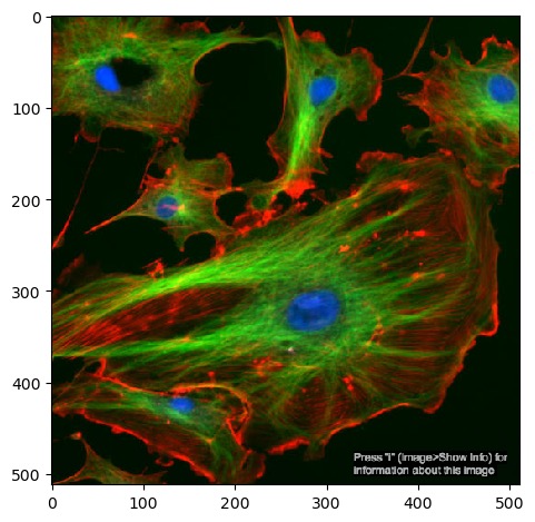
If we want to see what the image looks like, we need tell Python to
display it as an image. We can do this with the imshow
function from matplotlib, which you may already be familiar with as a
library for drawing plots and graphs, but it can also display
images.
PYTHON
import matplotlib.pyplot as plt

plt.set_cmap('gray')  # by default, single-channel images will now be displayed in greyscale
plt.imshow(image)
You should now see the image displayed below the current cell:
Since images are multi-dimensional arrays of numbers, we can apply statistical functions to them and extract some basic metrics. Numpy arrays have methods for several of these already, including the image’s shape, data type and minimum/maximum values:
PYTHON
print(image.shape, image.dtype, image.min(), image.max())
# returns: (512, 512, 3) uint8 0 255
This shows that the image has a data type of uint8, it contains
values between 0 and 255 and that it is in three dimensions. We can
reasonably infer that the two 512 numbers are the X and Y
axes. The third axis in most cases will represent a number of
channels.
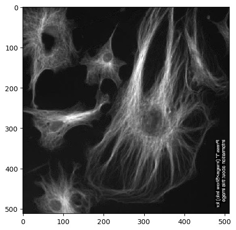
We can select a single channel by indexing the array:
Here, we select the entire X and Y axes using : with no
numbers around them, and the last channel (remember that Python counts
from 0).
Channels, series and stacks
Images can consist of more than two axes. The first two axes are usually X and Y, but if there is a third axis, then this could be one of several things:
- Channel - the image shows different features in the same 2D space. One common example is cell images with different staining for nuclei and membranes, expressed as different colours.
- Time series - the image is a collection of 2D frames taken at different points in time.
- Z-stack - essentially a series of 2D images piled up on top of each other in 3D space.
It’s usually easy enough to tell that you’re looking at a colour channel from looking at the image directly, but it may be more difficult to to distinguish a Z or a timepoint axis from the data alone. If you don’t know exactly how the images were generated, it’s a good idea to consult documentation or metadata.
Exercise 1: Loading an image
Load the test image ‘FluorescentCells_3channel.tif’:
- Try the same as the example above, but display one of the other channels
- Save your single channel to a variable. What happens if you run
imshowonchannel.T? - How can we select part of the image, i.e. crop it? Remember that to do this, we need to select a subset of the X and/or Y axes.
Other channels can be loaded with image[:, :, x], where
image is the variable the image is saved to and
x is the index of a channel to retrieve.
Next we can use .T to return a
transposed version of the image. Running
imshow() on this results in an image that is flipped
90°:
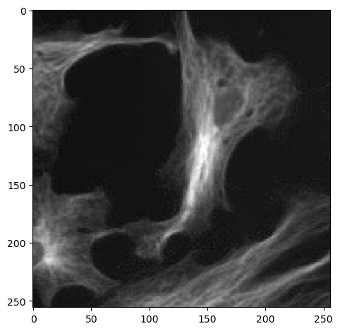
Remember that Numpy arrays can be sliced and indexed the same way as
lists, strings and tuples. Up to this point we’ve been using
: to select an entire axis, but we can give it start and
end bounds to select part of the X and Y axes, like:
Numpy arrays have many more methods available for checking them. Here are just a few to start with:
Object size
Note that some of these are functions and need to be called with
brackets(()), whereas others are simply attributes that do
not.
Exercise 2: Memory check
How much memory did it take to load FluorescentCells_3channel.tif?
Running image.nbytes shows that it takes up 786432
bytes, or ~786 kilobytes, or ~0.7 megabytes.
Displaying one channel at a time
We’ve seen from exercise 1 that we can view single channels by indexing the array. We can also show all channels together using a matplotlib figure:
PYTHON
import matplotlib.pyplot as plt
plt.figure(figsize=(12, 6))  # figure size, in inches
nchannels = 3

for i in range(nchannels):
    # Use subplot() to create a multi-image figure with 1 row and 3 columns. We need to increment i by 1
    # because range() counts from 0 but subplot() assumes you're counting from 1.
    plt.subplot(1, nchannels, i+1)
    plt.imshow(image[:, :, i])
    plt.title('Channel ' + str(i))  # add a plot title
    plt.axis(False)              # we just want to show the image, so turn off the axis labels

plt.show()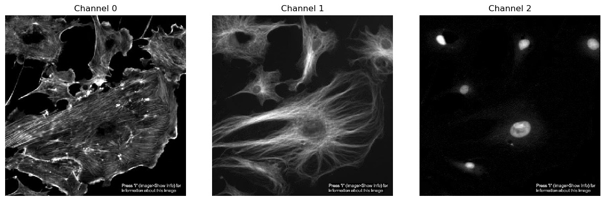
Histograms
Another useful metric in image analysis is an image’s histogram. This can be plotted by flattening the image and passing it to matplotlib:
First, we need to select a single channel - since different channels
may represent different cell organelles or points in time, we need to
ensure that we are comparing like with like. We also need
flatten() because we don’t care about the arrangement of
the pixels, we just want to sort their values values into bins. Finally,
we can use bins to control how many bins the data is split
into.
Exercise 3: Histograms
Combine the usage of matplotlib.pyplot.hist() and
matplotlib.pyplot.figure() introduced above above and plot
a histogram of each of the three channels in
FluorescentCells_3channel.tif.
Starting with displaying a single histogram for one channel:
PYTHON
channel_idx = 0
channel = image[:, :, channel_idx]
plt.hist(channel.flatten(), bins=255)
plt.title('Channel ' + str(channel_idx))
plt.show()
We could call this three times, each with a different value for
channel_idx, or we can use a for loop:
PYTHON
plt.figure(figsize=(12, 6))  # figure size, in inches
nchannels = image.shape[-1]

for i in range(nchannels):
    channel = image[:, :, i]

    plt.subplot(1, nchannels, i+1)
    plt.hist(channel.flatten(), bins=255)
    plt.title('Channel ' + str(i))  # add a plot title

plt.show()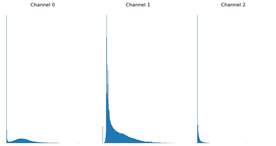
Proprietary formats
Modern microscopes save files in vendor-specific formats (like .czi, .nd2, or .lif). While skimage can handle standard TIF(F)s, these complex files contain vital metadata, for example, pixel spacing information, that we need for accurate analysis.
The Universal Adapter: BIOIO
Instead of installing a different library for every microscope brand, we recommend BIOIO. It acts as a consistent interface for almost any biological image format, allowing you to use the same commands regardless of the file source.
If using JupyterHub or JupyterLab, go to ‘New’ -> ‘Terminal’. This
will open a shell session in a new browser tab, where you can run
pip install commands.
Advanced: Scaling up with Dask
Once you are a bit more established as a Python user, the integration of BIOIO with Dask becomes a major advantage. It allows for “Lazy Loading,” where the computer only reads the specific pixels you ask for. This is essential for analyzing massive datasets that are larger than your computer’s RAM.
Exercise 4: Reading with BIOIO
Load the bioio package and use it to read the test file ‘data/Ersi_organoid_WT2.nd2’.
- Use print(img.dims) to check the dimensions. What does each letter represent?
- Use get_image_data to extract a single 2D frame for the first channel (C=0) at the middle Z-slice (Z=13).
PYTHON
from bioio import BioImage

# Load the image object
img = BioImage('data/Ersi_organoid_WT2.nd2')

# Check dimensions explicitly
print(img.dims)
# Returns: Dimensions [T: 1, C: 3, Z: 27, Y: 512, X: 512]

# Grab a specific slice (Channel 0, Z-slice 13)
pixel_data = img.get_image_data("YX", C=0, Z=13)

import matplotlib.pyplot as plt
plt.imshow(pixel_data)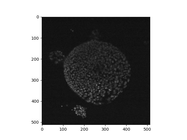
Altering the lookup table
Now that we have extracted a specific 2D slice of data using BIOIO, we can explore different ways to display it.
The imshow() function can take an argument called cmap, which applies a “Lookup Table” (LUT). This maps the numerical intensity values in your image to specific colors on your screen.
PYTHON
# Using the pixel_data we extracted from the BIOIO object earlier
plt.imshow(pixel_data, cmap='viridis')
Skimage uses lookup tables from the plotting library matplotlib. A list of available tables can be obtained with:
Exercise 5: Lookup tables
Go back to the FluorescentCells_3channel.tif image. Display each of
its three channels side by side in a matplotlib figure, each in a
different colour using cmap=. Use the values in
matplotlib.colormaps to select a lookup table for each
one.
There will be many ways to do this (and many colour maps to choose from!), but here is one possible solution:
PYTHON
# you'll need to run this again if you overwrote your `image` variable
image = imread('data/FluorescentCells_3channel.tif')
plt.figure(figsize=(12, 6))

plt.subplot(1, 3, 1)
plt.imshow(image[:, :, 0], cmap='Blues')

plt.subplot(1, 3, 2)
plt.imshow(image[:, :, 1], cmap='Oranges')

plt.subplot(1, 3, 3)
plt.imshow(image[:, :, 2], cmap='YlOrBr')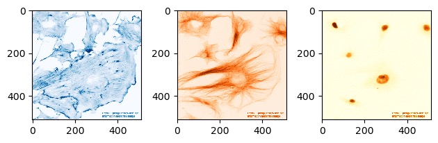
Exercise 5: Lookup tables (continued)
Load hela-cells_rgb.tif and try displaying it with different lookup tables. What results do you get? Why might this be the case?
The resulting image will not look as expected, and in Jupyter the image will appear unchanged. In this case, since the lookup table is being ignored, this would imply that the pixel values do not represent light intensities but rather are explicitly encoded colour values - i.e. it’s an RGB image.
Other notes
Rearranging channels
You may find yourself in a situation where the arrangement of
dimensions in your image is incorrect for the processing you wish to
perform on it - maybe a function requires that an image be oriented in a
particular way. This is where it’s useful to be able to rearrange the
dimensions of an image. To do this, we can use Numpy’s
moveaxis function:
PYTHON
import numpy
image = imread('data/FluorescentCells_3channel.tif')
print(image.shape)
# returns: (800, 800, 3)
rearranged_image = numpy.moveaxis(image, -1, 0)
print(rearranged_image.shape)
# returns: (3, 800, 800)
print(image.shape)
# returns: (800, 800, 3)
We can see that calling moveaxis on an array gives us a
rearranged version of the array given to it - the channel axis that was
at the end is now at the front. However, we can see that the original
value of the image is unchanged. This is because by default,
moveaxis returns a rearranged copy of the
image.
The arguments supplied are:
- The image or array
- The current position of the dimension to move
- The position to move that dimension to
In this case, we are moving the dimension at position -1 (i.e. the one at the end) to position 0 (the start).
Pixel size
To make real-world measurements, we need the image’s pixel size. While older methods required digging through complex metadata dictionaries, BIOIO makes this simple:
PYTHON
# Access the physical pixel sizes directly from the bioio object
print(img.physical_pixel_sizes)
# Returns physical sizes (e.g., X=0.1, Y=0.1, Z=0.5) usually in micrometres.Standard image formats (TIFF, PNG) can be loaded as NumPy arrays using skimage. Proprietary microscope formats are best handled by BIOIO to preserve dimensions and metadata. Basic metrics like histograms, shape, and pixel ranges help determine the best analysis strategy. Lookup tables (LUTs) change how data is rendered visually but do not change the underlying pixel values. Lazy loading (via Dask in BIOIO) allows you to explore massive datasets without overwhelming your computer’s memory.